Posts with «tutorial» label

Build your own drum pad

With the Drum kit – Kit AI by Spikenzielabs you can build an electronic drum kit. The bundle contains all of the electronics, including the piezo sensors for the drum pads. You build the drum pads yourself, and then connect the Drum Kit – Kit AI to your computer to play sounds using your favorite audio software, or use the MIDI-out port to a connected drum synthesizer.

Roberto De Nicolò (aka Rodenic) has realized an useful tutorial video showing what he has called FingerDrum. Roberto has applied a piezo sensor to each finger of a glove, allowing the triggering of individual drum sounds from his midi expander. If you think the glove is unconfortable, check out the FingerPad and turn your mouse pad into a drum pad.


Arduino Blog 17 Sep 14:38

How to make an Arduino shield with Eagle CAD – Tutorial

-->-->-->-->

There are many CAD developed to assist the electronic designers during drawing of PCBs and schematics; often they are integrated in complete suite to project, simulate and realize a whole electronic system. Besides the many commercial versions, there are also free CADs available. Today we’d like to analyze one of the most diffused and known software: Eaglecad (eagle does not mean the powerful bird but it is the acronym of Easily Applicable Graphical Layout Editor) made by Cadsoft, actually at version 6.2.0. We have chosen this one because, as you know as an Arduino’s fan, the official pcbs and schematic files of the boards are developed and available free of charge to everybody in Eaglecad format; you can find also a lot of libraries and circuits made by famous DIY website (Sparkfun for first) available for free. Eaglecad is a professional software that have gained a lot of popularity due to the Arduino’s success. One of the most important difference between Eaglecad and its competitors is the availability of a version for every of the most common desktop OS: Windows, Linux, Mac. We have to specify that Eaglecad is not Free software but is a commercial one, which can be used in the free version (eaglecad light) only for evaluation purposes and by student but you can’t use the light version in any case when you earn or save money by using it. For further details about licenses and distributors have a look to the official Eaglecad website where you can find all the information you need. Remember that the light version has some limitations; anyway you can design circuit with a discrete complexity, as the one you can see at http://elmicro.com/en/kit12.html. The limitations are:

 - pcb dimensions not bigger than 100×80 mm;

 - no more than 2 layers;

 - only 1 sheet for schematic.

Now let’s have a look at the software itself starting from the GUI, which is made by three main units:

Control Panel

Schematic (you can see an Arduino’s UNO R3 board schematic screenshot)

Board (the pcb editor) which can be seen “in action” which shows the pcb of the Arduino’s R3 board


For people used to the other similar cads, the interface is very closed to them and you’ll learn to use it easily; anyway to use the most powerful functions you need some practice.

The first thing you see at the CAD start up is the Control Panel, from which you can easily get access (for example) to the libraries, projects and examples; this is the software section where you can configure the main options like user’s folders, delay for the autosave option and the most important graphical parameters, all by getting access to the “OPTIONS” menu. The available documentation is pretty complete: you can access to the help function from the “help” menu available in both “Schematic” and “Pcb”. If you need further details you have to read the complete manual and the tutorial which are both available getting access to “Start” (on Windows), Programs-> Eagle Layout Editor 6.2.0.

Let’s try to have practice with an example: we want to draw an Arduino’s shield made by 4 leds e da 4 switches, connected to 8 digital pins; it’s obvious due to the kind of circuit we are approaching to make, that this shield is only for training purposes. This pcb can be used to show the digital logic level of one or some pins, levels that could be changed by the four switches or to have a led alarm in case of an analog becomes higher or lower than some level.

For first we have to draw the schematic so we select “FILE”, “NEW”, “SCHEMATIC” in this order: the Schematic window will open up. It is mainly made by two groups of icons: one on the top with the main commands like file management and zoom and another one on the left with the “drawing” icons.


We can add the components by selecting the “AND” gate icon on the left hand side of the screen; when the cursor will be on it the word “Add” will pop up. Once selected, a list of libraries will be shown.

We can add other libraries like the Sparkfun one for example or we can also modify the ones which are provided by Eaglecad. Now select “Resistor”, “R-EU”: on the screen will appear a sub library where we can choose the kind of resistor we need (SMD,trough-hole) and its package.

For our example we’d like to use trough hole components so we’ll choose “R-EU_02_07/10″ which is a 1/4W resistor horizontally mounted. Once a component has been chosen, on the right hand side of the window, Eaglecad shows the component symbol used in the schematic and beside the pcb pads of such component and the space required on the PCB. There is another window under the two we have seen before where there are details and notes that have been inserted during creation of the selected component.

We need 4 of such components so we click on “OK”, move on the schematic drawing area and put the element where we want by clicking again. Eaglecad automatically names resistors in a progressive way.

When we have finished with these components, we have to select “ESC” on the keyboard: again the “ADD” window will open itself; now we select “LED5MM” in the “LED” sub-library which is contained into the “Led” library and we’ll draw four leds as done before.

In the same way we can select the 4 switches “10-xx” available in the library “switch-omron”; these actions lead us to the situation shown here:

For the moment we can mainly focus our attention about the correct type of the connectors so we add, as explained before, two made by 6 contacts for the power supply section and the analog connections and other two made by 8 pins for digitals; the chosen connectors are the ones in the “con-molex” library, identified by “22-23-2061″ e “22-23-2081″. Push two times ESC to exit and so far we are in the conditions show:

Now select the 4 resistors one at time, right-click and select “Value” in order to assign the desired value to each of them. Do the same with the 4 connectors, in order to change their value e.g. into A1, A2, D1, D2. A warning window with two choices will pop up: we’ll chose “Yes” and in the next window we’ll insert the required value. We’ll do the same for the next three strips.

Now below every resistors there is the resistance value and also the four connectors have been renamed as required. It is also possible to rename every singol contact of every connector. Let’s do that, in order to avoid mistakes: select “name” in the left hand column and then put the mouse cursor on every contact to replace their name, e.g. “D1″, “D2″, “A1″, “A2″.

In this way it is easy to understand for every contact which is the related connector strip. Now insert the ground symbol and connect the LED cathodes to them (Eaglecad have available many kind of ground symbols: they are in the libraries “supply1″ and “supply2″). We’ll choose “GND” available in the “supply1″ library. Looking at the digital strips we can notice that they are in the “wrong” side of the schematic. To have a more easily access to the contact connections and to have a clear and readable schematic, we can use the”mirror” command to mirror the selected parts. Before apply this command, select the symbols of both connectors with the command “group” in order to reduce the number of required actions.

Select “Mirror” and then put the mouse pointer on the working area and select by left clicking first and then by right clicking “Mirror: Group”. Now it’ s time to draw connections. We can proceed in two ways: by selecting the commands “Draw” and “Wire” in sequence or by clicking with the left mouse switch on the related icon. To connect components put the cursor on the end of the symbol you want to connect, click with the left mouse switch and move the pointer on the terminal of the other components you have to connect to and click again.

To go to the next connection push ESC on the keyboard, put the mouse pointer where you want to draw the next wire and then left click again.

So far so good. We have focused our attention on LEDs, forgetting the switches. Never mind, we can insert, modify, delete, change the inserted parts in the schematic every time we need it; now we insert the missing components adding the required connections.

As you can see it’s easy to rotate and to move any part by using the related function in the “edit” menu or by selecting the desired icon in the left hand side column.

Once all the connections are done, select “Tool”, “Erc” to solve errors, if any, which will be shown in the “Erc errors” window where Eaglecad lists some issues: leds and switches have no value and the pins of the strips are not connected.

We don’t care about the missing values because they are not important in our schematic and we know that the unconnected pins are not used in our circuit. To confirm that, select “Approve” for all the requests and then with “Tools” and “”Errors” command we make sure that there are no further issues. Finally it’s time to draw the printed circuit board: left click on the “Board” icon which is the fifth starting from the left on the tool bar which is on the top of the working window.

The system will ask us if we want to create the related file so we confirm “Yes” and then we’ll have on the screen the same picture as the one shown in figure:

Using the command “Move” which can be selected by the icon with the four arrows in the left hand column, move the components where required. It’s better to start with the connectors due to they give the dimensions to the shield. Remember that the eight and the 6 pins connectors don’t have the same “step” on the board; in case of doubt check another shield, or you can refer to the pcb of the Uno which can be easily found on the Arduino’s website. The ones who have the R3 know that the strips have been redrawn to follow the increased needs of such system so the old connectors 8+8 and 6+6 have been replaced with 10+8 for digital pins and 8+6 for analog. In our example we have chosen to use the old connectors because they are compatible with all the Arduino version between 2009 and Uno and then because our shield was born for teaching reasons so it’s better to have it compatible also with the old pcb versions which are still used by many people. To insert the four connectors we can use the grid which help us; to change its resolution get access to “View”, “Grid” or “Properties” which is available by the “i” icon; in the last case we have also information about the absolute position in the working space.

Since the versions 6 of Eagleacad it is available another function which support us during drawing: “dimension” available through “Draw->Dimension”.

Wiring routing can be done automatically (autorouting function) or manually. In this short introduction we’ll use the hand routing in order to practice with Eaglecad. By selecting the “Route” icon it is possible to draw connections; the dimension, shape and width are visible on the top icon bar where is also possible to select the pcb side. The freeware version make possible to draw pcbs with only two sides, so we’ll find only “Top” and “Bottom”. In the same way you move components it is possible to define the printed circuit board dimensions; the white lines are the cutting boarder where the CNC will cut the pcb. Finally here a possible two sides pcb of our Arduino’s shield.

Special thanks to author Vincenzo Mendola.

-->-->-->-->-->-->
-->-->

Quick tutorial: current sensing for DC motors

On her blog, Dustyn Roberts presents her own experience on current sensing for controlling DC electric motors with an Arduino board and an Arduino Motor Shield. This shield, based on a L298 H-bridge, provides two current sensing pins to the user, which can be used to measure the instantaneous current absorpion by each H-bridge. After some trials, Dustyn managed to have a quite clear picture of the absorption behavior of the DC motor:

Sample code and updates can be found on Dustyn’s blog.

[Via: Dustyn's blog]

Insert Coin: Tabber lights up your fretboard, shows you the way to rock

In Insert Coin, we look at an exciting new tech project that requires funding before it can hit production. If you'd like to pitch a project, please send us a tip with "Insert Coin" as the subject line.
The idea of a lighted fretboard isn't a new one by any stretch (how do you think the Fretlight got its compound name?), but there's something to be said for not having to buy a brand new guitar for that functionality. The folks behind Tabber are working to make that a reality, having tested a number of prototypes for a product that you can simply slip over the neck of your axe for a quick tutorial. The company is looking to create a slicker version of the concept that it can bring to the market. Tabber's creators need your help to "transform the guitar industry," so naturally they've taken to Kickstarter, with a little under a month to hit their $45,000 goal. The Arduino-powered LED guitar instructor will connect to a mobile device via Bluetooth, accessing information to let you play along with songs, figure out chords and bend your fingers around some scales. Click the source link to send some cash Tabber's way, or to find out a bit more about the project.

Update: As a number of commenters have pointed out, there's a similar project currently awaiting your donations on Kickstarter. Great minds, huh?

Continue reading Insert Coin: Tabber lights up your fretboard, shows you the way to rock

Insert Coin: Tabber lights up your fretboard, shows you the way to rock originally appeared on Engadget on Thu, 22 Mar 2012 11:00:00 EST. Please see our terms for use of feeds.

Permalink | Email this | Comments

Arduino ISP (In System Programming) and stand-alone circuits

We use an Arduino to program other ATmega without bootloader . This technique allows you to use all flash memory for code and make boards using new ATmega, cheaper than those with bootloader.

The qualities that have made the success of Arduino are undoubtedly the open-source software, many libraries, a good hardware and a virtually infinite Reference that explains each possible use of the platform.

But if we use Arduino for a specific use, we can integrate it into a specific circuit and program the micro in a way that performs a single firmware. We may so remove the bootloader and leave to the firmware the entire program memory.

The ATmega328 has 32 Kbytes of flash, that when the chip is mounted on Arduino are not all available, as a portion is reserved to the bootloader, the purpose of which is to communicate with the IDE Arduino to load programs (sketch) to be performed. The same bootloader, on each power on or reset of Arduino, verifies the presence of a sketch in flash memory and executes it. The bootloader occupies a space of 512 bytes, in the case of Arduino UNO.

Well, in a stand-alone application the bootloader no longer needed.

The configuration of the micro ATmega328P needs, in addition to the power (+5 VDC to pins 7 and 20, GND to pins 8 and 22), a 16-MHz crystal between pins 9 and 10, two 22 pF ceramic capacitors from between these pins and GND, a 10 k Ω resistor between pin 1 and +5 VDC for pull-up the reset line.


Programming ATMEGA in stand-alone

Anyone knows that it is necessary program Arduino uploading a sketch via USB, using the software called IDE and the operation is quite simple.

We can see a screenshot of the IDE with an Arduino sketch loaded and UNO during the receipt of the sketch (notice the yellow LED on).

The technique will test allows the use of a board Arduino as ISP Programmer.

We start with the list of required materials:

•               Arduino UNO / Duemilanove (will be used as a programmer);

•               ATmega328P chip (chip to be programmed);

•               Breadboard and jumper;

•               a crystal of 16 MHz, two ceramic capacitors from 22 pF, a resistance of 10 K Ω 1/4 W, a resistance of 560 Ω 1/4 W LED 3 or 5 mm;

•               seven male-male jumper wires.

A resistance of 120 Ω 1/4 of watts, and an electrolytic capacitor or tantalum from 10 uF 10 ÷ 16 volts.


Now we prepare our target circuit and first of all insert the chip on the Breadboard, these are the connections to make:

•               through the jumper to be Breadboard connect pins 7 and 20 of the chip to the positive supply line (+5 volts);

•               in the same way we connect the pins 8 and 22 of the chip to the ground line supply (GND);

•               connect pin 1 of the chip to the +5 V line through the resistor of 10 k Ω;

•               insert the crystal to the pins 9 and 10 of the chip;

•               insert the two 22 pF ceramic capacitors; both must have a leg connected to GND, while the other will serve to connect a capacitor to pin 9 and the other to pin 10 of the chip;

•               insert one end of resistor 560 Ω at the pin 19 and the other end into an empty spot on the breadboard, and to this end we connect the anode LED(the longer pin) , whose other end (cathode) goes to GND;


At this point we can connect to the Arduino Breadboard using jumper cables under the following matches:

•               Arduino pin 10 goes to pin 1 of the chip;

•               Arduino pin 11 goes to pin 17 of the chip;

•               pin 12 of Arduino is connected to pin 18 of the chip;

•               pin 13 to Arduino pin 19 goes on the chip;

•               the +5 V pins of Arduino goes to the positive supply line of the breadboard;

•               any of the three GND pin of Arduino goes to the ground line of the breadboard.


Now look the software to reveal the “trick” that sends a sketch, using the IDE, to the chip on the Breadboard, bypassing Arduino that will play the role of Programmer ISP.

What we need to do is create a virtual board, starting from the original (corresponding to the model we are using Arduino) and making some simple but essential changes. We must first locate the file that is boards.txt containing all information relating to the various boards that the IDE shows us when we execute the command Tools->Board. Typically this file is located in the folder of the IDE software, the path X: \ mypath \ arduino-xxx \ hardware \ arduino, where X is the letter that indicates the logical drive and myPath the folder or location containing the program (xxx indicates the version of the program).

Now open the file with Notepad and see a long series of lines arranged in groups separated by a line consisting of a repetition of the symbol ”#”,each group representing a different board. The lines are identified by the initial code, the same for all, but different for the board, the name that will appear in the submenu Tools->Board is inserted in the first row in the group.

The code is represented by the word “uno” which is at the beginning of each line.

The line containing the word “name” (usually the first) is followed by “=” and then the name that the board will have in the IDE.

Other information that concern us are:

uno.upload.maximum_size = 32256: Sets the maximum capacity of flash memory that we can use in practice from 32 Kbytes of Flash which has the total ATmega328P we must subtract the space occupied by the bootloader, for the Arduino UNO is 512 byte;

uno.bootloader.low_fuses = 0xffuno.bootloader.high_fuses = 0xdeuno.bootloader.extended_fuses = 0×05; these three lines are the “fuse”, are used to set the behavior of the chip and are expressed with hexadecimal values;

uno.build.f_cpu = 16000000L: This line must correspond to the clock frequency for which the chip has been set, by means of the fused, expressed in Hz, 1 Hz 6,000,000 correspond to 16 MHz, precisely the frequency of the quartz or, more precisely, the present external oscillator to Arduino UNO; this value is used as a reference for timing controls of the software, such as delay () and millis ().


And now we create our own virtual board, writing these lines of code:


atmsa16.name=ATmega in Stand Alone (w/ Arduino as ISP)
atmsa16.upload.protocol=stk500
atmsa16.upload.maximum_size=32768
atmsa16.upload.speed=115200
atmsa16.upload.using=arduino:arduinoisp
atmsa16.bootloader.low_fuses=0xff
atmsa16.bootloader.high_fuses=0xdf
atmsa16.bootloader.extended_fuses=0x05
#### atmsa16.bootloader.extended_fuses=0x07
atmsa16.bootloader.path=optiboot
atmsa16.bootloader.file=optiboot_atmega328.hex
atmsa16.bootloader.unlock_bits=0x3F
atmsa16.bootloader.lock_bits=0x0F
atmsa16.build.mcu=atmega328p
atmsa16.build.f_cpu=16000000L
atmsa16.build.core=arduino


Following the approach of the file will separate this group of lines to those of other boards, inserting a line of ”#”.The end result should be:

We note that are varied: the code (atmsa16 instead of uno), the maximum_size (brought to its maximum capabilities of Flash, since we do not reserve space for the bootloader), then there a new line (atmsa16.upload.using = arduino: arduinoisp) that allows us to understand the IDE that will program the chip in stand-alone and not on the Arduino. Another new line is preceded by some “# # # #” that disables it, the reason is easily explained: the extended_fuses is set to 0×05, and in some special cases, during the transfer of the sketch could be an error bound the setting of this value.As we shall see later, simply change the following two lines of code:

 <em># # # # Atmsa16.bootloader.extended_fuses = 0x05</em>
<em>atmsa16.bootloader.extended_fuses = 0x0</em>7

thus activating the value 0×07 instead of 0×05, it will work out. Of course, this change should not be made before, but only if you get the error.


Program the micro

At this point we are ready for the final step: send our sketches to the chip mounted on the breadboard and then will test the operation separating it from Arduino.


To read the new board in the file, the IDE must be restarted, so if this program was open, when editing the file boards.txt must close it and restart it. To verify that our modification is successful, it is sufficient now run the command Tools->Board and check if there is now our “stand-alone” board, otherwise we should close the IDE and check the file boards.txt, because certainly we made ​​a mistake.

The technique used to send the sketch to the chip in stand-alone mode is very simple: First select the Arduino board that we are using as a programmer (eg Arduino Duemilanove or UNO) , just as we do for normal use of Arduino. Then select the Arduino serial port (the COM for Windows users) and recall from the IDE the sketch ArduinoISP, execute this command by clicking the Upload button on the IDE. After several seconds of the three flashing LEDs and Arduino to the breadboard of course (at the moment is physically connected to pin 13 of Arduino that, as we know, check out one of the three LEDs on the board) on the IDE will come the message “done uploading “.

Arduino is ready to play the role of Programmer ISP, select, now, our board IDE “ATmega Stand Alone (w / Arduino as ISP)“, without changing the COM.

We load the sketch “blink” and execute it again by clicking the Upload button on the IDE: LEDs and Arduino breadboard flash again, this time for a much shorter period, after which the IDE will show the message again “Done uploading”.

So our ATmega328P chip was programmed without having to physically fit on Arduino and now lives its own life. It is then ready to be mounted in the circuit which it is intended.

Of course, the chip can be reprogrammed at will with any kind of sketch.


Troubleshooting

At this point we have to solve three types of problem that may occur when we send the sketch to the chip stand-alone. The problems of’extended_fuses and of autoreset may occur on either Arduino Duemilanove or Arduino UNO, without that you can establish a certain rule.We must also emphasize that the remedies that will illustrate to 100% solve the problems, but must be applied only if the problem occurs.

We start from the situation that may occur if we use a blank chip, the Atmel set the fuse to make the chip work at 1 MHz with the internal oscillator. If we send a sketch directly, happens that the chip in stand-alone ignores the external crystal and times will be staggered: for example, the LED blink with the sketch will last about 16 seconds instead of 1 second. Simply, we set the fuse, the operation can be done easily by loading the bootloader on the chip before sending the sketch.

Before explaining this simple maneuver quickly clarify two points: the bootloader is sent once a chip virgin and will only serve to set the fuse, then it will become useless and the sketch overwrite it, if we had to first load the sketch, noticing the error, and then load the bootloader, no problem: the chip is set and we just have to resubmit the sketch. The simple steps that are going to describe will return very useful for cases where we wanted to prepare a blank chip to work directly on Arduino; is a good idea to have in the house a spare chip with bootloader of our board, so if you were unfortunately damaged the original, a simple substitution solves this problem immediately.

Here are the steps to follow:

•               prepare and connect the Breadboard Arduino as discussed previously;

•               We open the IDE and select the model we are using Arduino and port to which it is connected;

•               upload the sketch ArduinoISP to Arduino;

•               now execute the command Tools->Burn Bootloader w / Arduino as ISP;

•               After about a minute we loaded into the stand-alone chip the bootloader of Arduino boards (you may have noticed that in the IDE we’ve set our Arduino board).


As mentioned, the chip can be quickly mounted to receive the Arduino sketch, or leave it on the breadboard and repeat/execute the operation of sending the sketch stand-alone, this time the Blink will work perfectly.

Of course, other errors may occur, do not worry, keep reading this section and of course everything will be resolved.

So let the problem of ’extended_fuses: the rows of our virtual board we expected a double value for this cast, because it can happen (even though it is quite rare) that some boards do not succeed in this program merged with the value 0×05. During the upload of the sketch on the chip with stand-alone mode, the IDE will display an error message (written in red on a black background) that will indicate the need to use the value 0×07, if it appears that in practice warning means that we must close the IDE, open the file boards.txt and activate the relevant line, simultaneously disabling the other (with 0×05), as explained above. At this point we can repeat the test. We clarify that if the error occurs on a given board will always occur on this board, so the variation of the files should be done only once and permanently.

And now we see the problem, more frequent, about autoreset. When the serial chip (FT232RL on Duemilanove or ATmega8U2 of UNO) receives a signal from the USB port, sends the reset pulse to ATmega328, who then prepares itself to receive Data. This operation corresponds to the one you make every time you press the button “RESET” on the Arduino.

If the data do not arrive or if the reset was made manually, the sketches in flash memory chip ATmega328 is executed. When Arduino is used as ISP Programmer can happen that, if the autoreset is sent too early, the upload operation fails. In this case the IDE returns the following error: ”avrdude:stk500_getsync (): not in sync: resp = 0×15“.

The problem is solved by blocking the Autoreset. The 120 ohm resistance must be connected between the RESET pin of Arduino and +5 V, while the 10µF capacitor is connected with the positive pole to the RESET of Arduino and negative to GND.

With a jumper cable connect on Breadboard the RESET signal of Arduino.

The methods described should be used only if absolutely necessary.

Important note: the need to connect these components only when needed, is dictated by the fact that to load a sketch on the Arduino should autoreset, otherwise the upload will fail and we will get the error avrdude: stk500_getsync (): not in sync: resp = 0×00 – avrdude: stk500_disable (): protocol error, expect = 0×14, resp = 0×51, so if you see this error, know that you just have to “liberate” the pin “RESET” Arduino from the link with the Anti- autoreset.

[Thanks to Michele Menniti]

Neural Network (Part 7) : Cut and Paste Code

Ok - so you don't like tutorials, and would rather just cut and paste some code.
This is for you.
http://www.openprocessing.org/visuals/?visualID=33991

Make sure to select "Source code" when you get there, otherwise it will be quite boring.
Here is an animated gif which shows the program in action.


See BELOW for the WHOLE screenshot so that you don't have to speed read.


If you want to know how it works, then you will have to go back and read part 1 to 6.


  • Neural Network


  • But as you can see from the example above:
    Before the neural network is trained, the outputs are not even close to the expected outputs. After training, the neural network produces the desired results (or very close to it).

    Please note, this neural network also allows more than one output neuron, so you are not limited to single yes no decisions. You can use this neural network to make classifications. You will soon see this with my LED colour sensor.

    Feel free to use this Neural Network in your own projects, but please let me know if you do, just for curiosity sake.

    Update: See below for the Processing Sketch (much easier than going to the open processing site). It is a bit long - but saves you from having to navigate to another site.

    Processing sketch

      1
    2
    3
    4
    5
    6
    7
    8
    9
    10
    11
    12
    13
    14
    15
    16
    17
    18
    19
    20
    21
    22
    23
    24
    25
    26
    27
    28
    29
    30
    31
    32
    33
    34
    35
    36
    37
    38
    39
    40
    41
    42
    43
    44
    45
    46
    47
    48
    49
    50
    51
    52
    53
    54
    55
    56
    57
    58
    59
    60
    61
    62
    63
    64
    65
    66
    67
    68
    69
    70
    71
    72
    73
    74
    75
    76
    77
    78
    79
    80
    81
    82
    83
    84
    85
    86
    87
    88
    89
    90
    91
    92
    93
    94
    95
    96
    97
    98
    99
    100
    101
    102
    103
    104
    105
    106
    107
    108
    109
    110
    111
    112
    113
    114
    115
    116
    117
    118
    119
    120
    121
    122
    123
    124
    125
    126
    127
    128
    129
    130
    131
    132
    133
    134
    135
    136
    137
    138
    139
    140
    141
    142
    143
    144
    145
    146
    147
    148
    149
    150
    151
    152
    153
    154
    155
    156
    157
    158
    159
    160
    161
    162
    163
    164
    165
    166
    167
    168
    169
    170
    171
    172
    173
    174
    175
    176
    177
    178
    179
    180
    181
    182
    183
    184
    185
    186
    187
    188
    189
    190
    191
    192
    193
    194
    195
    196
    197
    198
    199
    200
    201
    202
    203
    204
    205
    206
    207
    208
    209
    210
    211
    212
    213
    214
    215
    216
    217
    218
    219
    220
    221
    222
    223
    224
    225
    226
    227
    228
    229
    230
    231
    232
    233
    234
    235
    236
    237
    238
    239
    240
    241
    242
    243
    244
    245
    246
    247
    248
    249
    250
    251
    252
    253
    254
    255
    256
    257
    258
    259
    260
    261
    262
    263
    264
    265
    266
    267
    268
    269
    270
    271
    272
    273
    274
    275
    276
    277
    278
    279
    280
    281
    282
    283
    284
    285
    286
    287
    288
    289
    290
    291
    292
    293
    294
    295
    296
    297
    298
    299
    300
    301
    302
    303
    304
    305
    306
    307
    308
    309
    310
    311
    312
    313
    314
    315
    316
    317
    318
    319
    320
    321
    322
    323
    324
    325
    326
    327
    328
    329
    330
    331
    332
    333
    334
    335
    336
    337
    338
    339
    340
    341
    342
    343
    344
    345
    346
    347
    348
    349
    350
    351
    352
    353
    354
    355
    356
    357
    358
    359
    360
    361
    362
    363
    364
    365
    366
    367
    368
    369
    370
    371
    372
    373
    374
    375
    376
    377
    378
    379
    380
    381
    382
    383
    384
    385
    386
    387
    388
    389
    390
    391
    392
    393
    394
    395
    396
    397
    398
    399
    400
    401
    402
    403
    404
    405
    406
    407
    408
    409
    410
    411
    412
    413
    414
    415
    416
    417
    418
    419
    420
    421
    422
    423
    424
    425
    426
    427
    428
    429
    430
    431
    432
    433
    434
    435
    436
    437
    438
    439
    440
    441
    442
    443
    444
    445
    446
    447
    448
    449
    450
    451
    452
    453
    454
    455
    456
    457
    458
    459
    460
    461
    462
    463
    464
    465
    466
    467
    468
    469
    470
    471
    472
    473
    474
    475
    476
    477
    478
    479
    480
    481
    482
    483
    484
    485
    486
    487
    488
    489
    490
    491
    492
    493
    494
    495
    496
    497
    498
    499
    500
    501
    502
    503
    504
    505
    506
    507
    508
    509
    510
    511
    512
    513
    514
    515
    516
    517
    518
    519
    520
    521
    522
    523
    524
    525
    526
    527
    528
    529
    530
    531
    532
    533
    534
    535
    536
    537
    538
    539
    540
    541
    542
    543
    544
    545
    546
    547
    548
    549
    550
    551
    552
    553
    554
    555
    556
    557
    558
    559
    560
    561
    562
    563
    564
    565
    566
    567
    568
    569
    570
    571
    572
    573
    /*Neural Network created by ScottC on 15th Aug 2011

    Please visit my blog for a detailed explanation of my Neural Network
    http://arduinobasics.blogspot.com/p/arduinoprojects.html

    */


    void setup(){
    ArrayList myTrainingInputs = new ArrayList();
    ArrayList myTrainingOutputs = new ArrayList();

    float[] myInputsA={0,0};
    float[] myInputsB={0,1};
    float[] myInputsC={1,0};
    float[] myInputsD={1,1};
    float[] myOutputsA={1};
    float[] myOutputsB={0};


    println("TRAINING DATA");
    println("--------------------------------------------");
    myTrainingInputs.add(myInputsA);
    myTrainingOutputs.add(myOutputsA);
    println("INPUTS= " + myInputsA[0] + ", " + myInputsA[1] + "; Expected output = " + myOutputsA[0]);
    myTrainingInputs.add(myInputsB);
    myTrainingOutputs.add(myOutputsB);
    println("INPUTS= " + myInputsB[0] + ", " + myInputsB[1] + "; Expected output = " + myOutputsB[0]);
    myTrainingInputs.add(myInputsC);
    myTrainingOutputs.add(myOutputsB);
    println("INPUTS= " + myInputsC[0] + ", " + myInputsC[1] + "; Expected output = " + myOutputsB[0]);
    myTrainingInputs.add(myInputsD);
    myTrainingOutputs.add(myOutputsA);
    println("INPUTS= " + myInputsD[0] + ", " + myInputsD[1] + "; Expected output = " + myOutputsA[0]);
    println("--------------------------------------------");

    NeuralNetwork NN = new NeuralNetwork();
    NN.addLayer(2,2);
    NN.addLayer(2,1);

    println("Before Training");
    float[] myInputDataA1={0,0};
    NN.processInputsToOutputs(myInputDataA1);
    float[] myOutputDataA1={};
    myOutputDataA1=NN.getOutputs();
    println("Feed Forward: INPUT = 0,0; OUTPUT=" + myOutputDataA1[0]);

    float[] myInputDataB1={0,1};
    NN.processInputsToOutputs(myInputDataB1);
    float[] myOutputDataB1={};
    myOutputDataB1=NN.getOutputs();
    println("Feed Forward: INPUT = 0,1; OUTPUT=" + myOutputDataB1[0]);

    float[] myInputDataC1={1,0};
    NN.processInputsToOutputs(myInputDataC1);
    float[] myOutputDataC1={};
    myOutputDataC1=NN.getOutputs();
    println("Feed Forward: INPUT = 1,0; OUTPUT=" + myOutputDataC1[0]);

    float[] myInputDataD1={1,1};
    NN.processInputsToOutputs(myInputDataD1);
    float[] myOutputDataD1={};
    myOutputDataD1=NN.getOutputs();
    println("Feed Forward: INPUT = 1,1; OUTPUT=" + myOutputDataD1[0]);

    println("");
    println("--------------------------------------------");

    println("Begin Training");
    NN.autoTrainNetwork(myTrainingInputs,myTrainingOutputs,0.0001,500000);
    println("");
    println("End Training");
    println("");
    println("--------------------------------------------");
    println("Test the neural network");
    float[] myInputDataA2={0,0};
    NN.processInputsToOutputs(myInputDataA2);
    float[] myOutputDataA2={};
    myOutputDataA2=NN.getOutputs();
    println("Feed Forward: INPUT = 0,0; OUTPUT=" + myOutputDataA2[0]);

    float[] myInputDataB2={0,1};
    NN.processInputsToOutputs(myInputDataB2);
    float[] myOutputDataB2={};
    myOutputDataB2=NN.getOutputs();
    println("Feed Forward: INPUT = 0,1; OUTPUT=" + myOutputDataB2[0]);

    float[] myInputDataC2={1,0};
    NN.processInputsToOutputs(myInputDataC2);
    float[] myOutputDataC2={};
    myOutputDataC2=NN.getOutputs();
    println("Feed Forward: INPUT = 1,0; OUTPUT=" + myOutputDataC2[0]);

    float[] myInputDataD2={1,1};
    NN.processInputsToOutputs(myInputDataD2);
    float[] myOutputDataD2={};
    myOutputDataD2=NN.getOutputs();
    println("Feed Forward: INPUT = 1,1; OUTPUT=" + myOutputDataD2[0]);


    }


    /* ---------------------------------------------------------------------
    A connection determines how much of a signal is passed through to the neuron.
    -------------------------------------------------------------------- */

    class Connection{
    float connEntry;
    float weight;
    float connExit;

    //This is the default constructor for an Connection
    Connection(){
    randomiseWeight();
    }

    //A custom weight for this Connection constructor
    Connection(float tempWeight){
    setWeight(tempWeight);
    }

    //Function to set the weight of this connection
    void setWeight(float tempWeight){
    weight=tempWeight;
    }

    //Function to randomise the weight of this connection
    void randomiseWeight(){
    setWeight(random(2)-1);
    }

    //Function to calculate and store the output of this Connection
    float calcConnExit(float tempInput){
    connEntry = tempInput;
    connExit = connEntry * weight;
    return connExit;
    }
    }


    /* -----------------------------------------------------------------
    A neuron does all the processing and calculation to convert an input into an output
    --------------------------------------------------------------------- */

    class Neuron{
    Connection[] connections={};
    float bias;
    float neuronInputValue;
    float neuronOutputValue;
    float deltaError;

    //The default constructor for a Neuron
    Neuron(){
    }

    /*The typical constructor of a Neuron - with random Bias and Connection weights */
    Neuron(int numOfConnections){
    randomiseBias();
    for(int i=0; i<numOfConnections; i++){
    Connection conn = new Connection();
    addConnection(conn);
    }
    }

    //Function to add a Connection to this neuron
    void addConnection(Connection conn){
    connections = (Connection[]) append(connections, conn);
    }

    /* Function to return the number of connections associated with this neuron.*/
    int getConnectionCount(){
    return connections.length;
    }

    //Function to set the bias of this Neron
    void setBias(float tempBias){
    bias = tempBias;
    }

    //Function to randomise the bias of this Neuron
    void randomiseBias(){
    setBias(random(1));
    }

    /*Function to convert the inputValue to an outputValue
    Make sure that the number of connEntryValues matches the number of connections */

    float getNeuronOutput(float[] connEntryValues){
    if(connEntryValues.length!=getConnectionCount()){
    println("Neuron Error: getNeuronOutput() : Wrong number of connEntryValues");
    exit();
    }

    neuronInputValue=0;

    /* First SUM all of the weighted connection values (connExit) attached to this neuron. This becomes the neuronInputValue. */
    for(int i=0; i<getConnectionCount(); i++){
    neuronInputValue+=connections[i].calcConnExit(connEntryValues[i]);
    }

    //Add the bias to the Neuron's inputValue
    neuronInputValue+=bias;

    /* Send the inputValue through the activation function to produce the Neuron's outputValue */
    neuronOutputValue=Activation(neuronInputValue);

    //Return the outputValue
    return neuronOutputValue;
    }

    //Activation function
    float Activation(float x){
    float activatedValue = 1 / (1 + exp(-1 * x));
    return activatedValue;
    }

    }

    class Layer{
    Neuron[] neurons = {};
    float[] layerINPUTs={};
    float[] actualOUTPUTs={};
    float[] expectedOUTPUTs={};
    float layerError;
    float learningRate;


    /* This is the default constructor for the Layer */
    Layer(int numberConnections, int numberNeurons){
    /* Add all the neurons and actualOUTPUTs to the layer */
    for(int i=0; i<numberNeurons; i++){
    Neuron tempNeuron = new Neuron(numberConnections);
    addNeuron(tempNeuron);
    addActualOUTPUT();
    }
    }


    /* Function to add an input or output Neuron to this Layer */
    void addNeuron(Neuron xNeuron){
    neurons = (Neuron[]) append(neurons, xNeuron);
    }


    /* Function to get the number of neurons in this layer */
    int getNeuronCount(){
    return neurons.length;
    }


    /* Function to increment the size of the actualOUTPUTs array by one. */
    void addActualOUTPUT(){
    actualOUTPUTs = (float[]) expand(actualOUTPUTs,(actualOUTPUTs.length+1));
    }


    /* Function to set the ENTIRE expectedOUTPUTs array in one go. */
    void setExpectedOUTPUTs(float[] tempExpectedOUTPUTs){
    expectedOUTPUTs=tempExpectedOUTPUTs;
    }


    /* Function to clear ALL values from the expectedOUTPUTs array */
    void clearExpectedOUTPUT(){
    expectedOUTPUTs = (float[]) expand(expectedOUTPUTs, 0);
    }


    /* Function to set the learning rate of the layer */
    void setLearningRate(float tempLearningRate){
    learningRate=tempLearningRate;
    }


    /* Function to set the inputs of this layer */
    void setInputs(float[] tempInputs){
    layerINPUTs=tempInputs;
    }


    /* Function to convert ALL the Neuron input values into Neuron output values in this layer, through a special activation function. */
    void processInputsToOutputs(){

    /* neuronCount is used a couple of times in this function. */
    int neuronCount = getNeuronCount();

    /* Check to make sure that there are neurons in this layer to process the inputs */
    if(neuronCount>0) {
    /* Check to make sure that the number of inputs matches the number of Neuron Connections. */
    if(layerINPUTs.length!=neurons[0].getConnectionCount()){
    println("Error in Layer: processInputsToOutputs: The number of inputs do NOT match the number of Neuron connections in this layer");
    exit();
    } else {
    /* The number of inputs are fine : continue
    Calculate the actualOUTPUT of each neuron in this layer,
    based on their layerINPUTs (which were previously calculated).
    Add the value to the layer's actualOUTPUTs array. */
    for(int i=0; i<neuronCount;i++){
    actualOUTPUTs[i]=neurons[i].getNeuronOutput(layerINPUTs);
    }
    }
    }else{
    println("Error in Layer: processInputsToOutputs: There are no Neurons in this layer");
    exit();
    }
    }


    /* Function to get the error of this layer */
    float getLayerError(){
    return layerError;
    }


    /* Function to set the error of this layer */
    void setLayerError(float tempLayerError){
    layerError=tempLayerError;
    }


    /* Function to increase the layerError by a certain amount */
    void increaseLayerErrorBy(float tempLayerError){
    layerError+=tempLayerError;
    }


    /* Function to calculate and set the deltaError of each neuron in the layer */
    void setDeltaError(float[] expectedOutputData){
    setExpectedOUTPUTs(expectedOutputData);
    int neuronCount = getNeuronCount();
    /* Reset the layer error to 0 before cycling through each neuron */
    setLayerError(0);
    for(int i=0; i<neuronCount;i++){
    neurons[i].deltaError = actualOUTPUTs[i]*(1-actualOUTPUTs[i])*(expectedOUTPUTs[i]-actualOUTPUTs[i]);

    /* Increase the layer Error by the absolute difference between the calculated value (actualOUTPUT) and the expected value (expectedOUTPUT). */
    increaseLayerErrorBy(abs(expectedOUTPUTs[i]-actualOUTPUTs[i]));
    }
    }


    /* Function to train the layer : which uses a training set to adjust the connection weights and biases of the neurons in this layer */
    void trainLayer(float tempLearningRate){
    setLearningRate(tempLearningRate);

    int neuronCount = getNeuronCount();

    for(int i=0; i<neuronCount;i++){
    /* update the bias for neuron[i] */
    neurons[i].bias += (learningRate * 1 * neurons[i].deltaError);

    /* update the weight of each connection for this neuron[i] */
    for(int j=0; j<neurons[i].getConnectionCount(); j++){
    neurons[i].connections[j].weight += (learningRate * neurons[i].connections[j].connEntry * neurons[i].deltaError);
    }
    }
    }
    }

    /* -------------------------------------------------------------
    The Neural Network class is a container to hold and manage all the layers
    ---------------------------------------------------------------- */

    class NeuralNetwork{
    Layer[] layers = {};
    float[] arrayOfInputs={};
    float[] arrayOfOutputs={};
    float learningRate;
    float networkError;
    float trainingError;
    int retrainChances=0;

    NeuralNetwork(){
    /* the default learning rate of a neural network is set to 0.1, which can changed by the setLearningRate(lR) function. */
    learningRate=0.1;
    }


    /* Function to add a Layer to the Neural Network */
    void addLayer(int numConnections, int numNeurons){
    layers = (Layer[]) append(layers, new Layer(numConnections,numNeurons));
    }


    /* Function to return the number of layers in the neural network */
    int getLayerCount(){
    return layers.length;
    }


    /* Function to set the learningRate of the Neural Network */
    void setLearningRate(float tempLearningRate){
    learningRate=tempLearningRate;
    }


    /* Function to set the inputs of the neural network */
    void setInputs(float[] tempInputs){
    arrayOfInputs=tempInputs;
    }


    /* Function to set the inputs of a specified layer */
    void setLayerInputs(float[] tempInputs, int layerIndex){
    if(layerIndex>getLayerCount()-1){
    println("NN Error: setLayerInputs: layerIndex=" + layerIndex + " exceeded limits= " + (getLayerCount()-1));
    } else {
    layers[layerIndex].setInputs(tempInputs);
    }
    }


    /* Function to set the outputs of the neural network */
    void setOutputs(float[] tempOutputs){
    arrayOfOutputs=tempOutputs;
    }


    /* Function to return the outputs of the Neural Network */
    float[] getOutputs(){
    return arrayOfOutputs;
    }


    /* Function to process the Neural Network's input values and convert them to an output pattern using ALL layers in the network */
    void processInputsToOutputs(float[] tempInputs){
    setInputs(tempInputs);

    /* Check to make sure that the number of NeuralNetwork inputs matches the Neuron Connection Count in the first layer. */
    if(getLayerCount()>0){
    if(arrayOfInputs.length!=layers[0].neurons[0].getConnectionCount()){
    println("NN Error: processInputsToOutputs: The number of inputs do NOT match the NN");
    exit();
    } else {
    /* The number of inputs are fine : continue */
    for(int i=0; i<getLayerCount(); i++){

    /*Set the INPUTs for each layer: The first layer gets it's input data from the NN, whereas the 2nd and subsequent layers get their input data from the previous layer's actual output. */
    if(i==0){
    setLayerInputs(arrayOfInputs,i);
    } else {
    setLayerInputs(layers[i-1].actualOUTPUTs, i);
    }

    /* Now that the layer has had it's input values set, it can now process this data, and convert them into an output using the layer's neurons. The outputs will be used as inputs in the next layer (if available). */
    layers[i].processInputsToOutputs();
    }
    /* Once all the data has filtered through to the end of network, we can grab the actualOUTPUTs of the LAST layer
    These values become or will be set to the NN output values (arrayOfOutputs), through the setOutputs function call. */
    setOutputs(layers[getLayerCount()-1].actualOUTPUTs);
    }
    }else{
    println("Error: There are no layers in this Neural Network");
    exit();
    }
    }


    /* Function to train the entire network using an array. */
    void trainNetwork(float[] inputData, float[] expectedOutputData){
    /* Populate the ENTIRE network by processing the inputData. */
    processInputsToOutputs(inputData);

    /* train each layer - from back to front (back propagation) */
    for(int i=getLayerCount()-1; i>-1; i--){
    if(i==getLayerCount()-1){
    layers[i].setDeltaError(expectedOutputData);
    layers[i].trainLayer(learningRate);
    networkError=layers[i].getLayerError();
    } else {
    /* Calculate the expected value for each neuron in this layer (eg. HIDDEN LAYER) */
    for(int j=0; j<layers[i].getNeuronCount(); j++){
    /* Reset the delta error of this neuron to zero. */
    layers[i].neurons[j].deltaError=0;
    /* The delta error of a hidden layer neuron is equal to the SUM of [the PRODUCT of the connection.weight and error of the neurons in the next layer(eg OUTPUT Layer)]. */
    /* Connection#1 of each neuron in the output layer connect with Neuron#1 in the hidden layer */
    for(int k=0; k<layers[i+1].getNeuronCount(); k++){
    layers[i].neurons[j].deltaError += (layers[i+1].neurons[k].connections[j].weight * layers[i+1].neurons[k].deltaError);
    }
    /* Now that we have the sum of Errors x weights attached to this neuron. We must multiply it by the derivative of the activation function. */
    layers[i].neurons[j].deltaError *= (layers[i].neurons[j].neuronOutputValue * (1-layers[i].neurons[j].neuronOutputValue));
    }
    /* Now that you have all the necessary fields populated, you can now Train this hidden layer and then clear the Expected outputs, ready for the next round. */
    layers[i].trainLayer(learningRate);
    layers[i].clearExpectedOUTPUT();
    }
    }
    }


    /* Function to train the entire network, using an array of input and expected data within an ArrayList */
    void trainingCycle(ArrayList trainingInputData, ArrayList trainingExpectedData, Boolean trainRandomly){
    int dataIndex;

    /* re-initialise the training Error with every cycle */
    trainingError=0;

    /* Cycle through the training data either randomly or sequentially */
    for(int i=0; i<trainingInputData.size(); i++){
    if(trainRandomly){
    dataIndex=(int) (random(trainingInputData.size()));
    } else {
    dataIndex=i;
    }

    trainNetwork((float[]) trainingInputData.get(dataIndex),(float[]) trainingExpectedData.get(dataIndex));

    /* Use the networkError variable which is calculated at the end of each individual training session to calculate the entire trainingError. */
    trainingError+=abs(networkError);
    }
    }


    /* Function to train the network until the Error is below a specific threshold */
    void autoTrainNetwork(ArrayList trainingInputData, ArrayList trainingExpectedData, float trainingErrorTarget, int cycleLimit){
    trainingError=9999;
    int trainingCounter=0;


    /* cycle through the training data until the trainingError gets below trainingErrorTarget (eg. 0.0005) or the training cycles have exceeded the cycleLimit

    variable (eg. 10000). */
    while(trainingError>trainingErrorTarget && trainingCounter<cycleLimit){

    /* re-initialise the training Error with every cycle */
    trainingError=0;

    /* Cycle through the training data randomly */
    trainingCycle(trainingInputData, trainingExpectedData, true);

    /* increment the training counter to prevent endless loop */
    trainingCounter++;
    }

    /* Due to the random nature in which this neural network is trained. There may be occasions when the training error may drop below the threshold
    To check if this is the case, we will go through one more cycle (but sequentially this time), and check the trainingError for that cycle
    If the training error is still below the trainingErrorTarget, then we will end the training session.
    If the training error is above the trainingErrorTarget, we will continue to train. It will do this check a Maximum of 9 times. */
    if(trainingCounter<cycleLimit){
    trainingCycle(trainingInputData, trainingExpectedData, false);
    trainingCounter++;

    if(trainingError>trainingErrorTarget){
    if (retrainChances<10){
    retrainChances++;
    autoTrainNetwork(trainingInputData, trainingExpectedData,trainingErrorTarget, cycleLimit);
    }
    }

    } else {
    println("CycleLimit has been reached. Has been retrained " + retrainChances + " times. Error is = " + trainingError);
    }
    }
    }
    The above code was formatted using hilite.me

    Neural Network (Part 6) : Back Propagation, a worked example

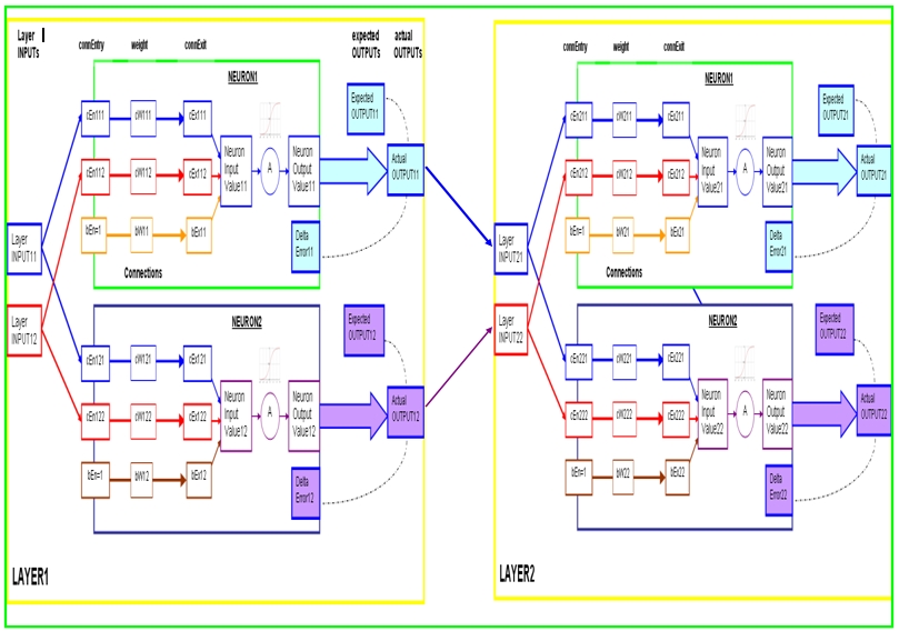
    A worked example of a Back-propagation training cycle.


    In this example we will create a 2 layer network (as seen above), to accept 2 readings, and produce 2 outputs. The readings are (0,1) and the expectedOutputs in this example are (1,0).

    Step 1: Create the network

    NeuralNetwork NN = new NeuralNetwork();   
    NN.addLayer(2,2);
    NN.addLayer(2,2);
    float[] readings = {0,1};
    float[] expectedOutputs = {1,0};
    NN.trainNetwork(readings,expectedOutputs);

    This neural network will have randomised weights and biases when created.
    Let us assume that the network generates the following random variables:

    LAYER1.Neuron1
    Layer1.Neuron1.Connection1.weight = cW111 = 0.3
    Layer1.Neuron1.Connection2.weight = cW112 = 0.8
    Layer1.Neuron1.Bias = bW11 = 0.5

    LAYER1.Neuron2
    Layer1.Neuron2.Connection1.weight = cW121 =  0.1
    Layer1.Neuron2.Connection2.weight = cW122 =  0.1
    Layer1.Neuron2.Bias = bW12 = 0.2

    LAYER2.Neuron1
    Layer2.Neuron1.Connection1.weight = cW211 = 0.6
    Layer2.Neuron1.Connection2.weight = cW212 = 0.4
    Layer2.Neuron1.Bias = bW21 = 0.4

    LAYER2.Neuron2
    Layer2.Neuron2.Connection1.weight = cW221 = 0.9
    Layer2.Neuron2.Connection2.weight = cW222 = 0.9
    Layer2.Neuron2.Bias = bW22 = 0.5


    Step 2: Process the Readings through the Neural Network

    a) Provide the Readings to the first layer, and calculate the neuron outputs

    The readings provided to the neural network is (0,1), which go straight through to the first layer (layer1).
    Starting with Layer 1:
    Layer1.INPUT1 = 0
    Layer1.INPUT2 =1

       Calculate Layer1.Neuron1.NeuronOutput
       ConnExit (cEx111) = ConnEntry (cEn111)  x Weight (cW111) = 0 x 0.3 = 0;
       ConnExit (cEx112) = ConnEntry (cEn112)  x Weight (cW112) = 1 x 0.8 = 0.8;
       Bias (bEx11) = ConnEntry (1) x Weight (bW11) = 1 x 0.4 = 0.4
       NeuronInputValue11 = 0 + 0.8 + 0.4 = 1.2
       NeuronOutputValue11 = 1/(1+EXP(-1 x 1.2)) = 0.768525
      
      Calculate Layer1.Neuron2.NeuronOutput
       ConnExit (cEx121) = ConnEntry (cEn121)  x Weight (cW121) = 0 x 0.1 = 0;
       ConnExit (cEx122) = ConnEntry (cEn122)  x Weight (cW122) = 1 x 0.1 = 0.1;
       Bias (bEx12) = ConnEntry (1) x Weight (bW12) = 1 x 0.2 = 0.2
       NeuronInputValue12 = 0 + 0.1 + 0.2 = 0.3
       NeuronOutputValue12 = 1/(1+EXP(-1 x 0.3)) = 0.574443


    b) Provide LAYER2 with Layer 1 Outputs.

    Now lets move to  Layer 2:
    Layer2.INPUT1 = NeuronOutputValue11 = 0.768525
    Layer2.INPUT2 = NeuronOutputValue12 = 0.574443

       Calculate Layer2.Neuron1.NeuronOutput
       ConnExit (cEx211) = (cEn211)  x Weight (cW211) = 0.768525 x 0.6 = 0.461115;
       ConnExit (cEx212) = (cEn212)  x Weight (cW212) = 0.574443 x 0.4 = 0.229777;
       Bias (bEx21) = ConnEntry (1) x Weight (bW21) = 1 x 0.4 = 0.4
       NeuronInputValue21 = 0.461115 + 0.229777 + 0.4 = 1.090892
       NeuronOutputValue21 = 1/(1+EXP(-1 x 1.090892)) = 0.74855
      
      Calculate Layer2.Neuron2.NeuronOutput
       ConnExit (cEx221) = (cEn221)  x Weight (cW221) = 0.768525  x 0.1 = 0.076853;
       ConnExit (cEx222) = (cEn222)  x Weight (cW222) = 0.574443  x 0.1 = 0.057444;
       Bias(bEx22) = ConnEntry (1) x Weight (bW22) = 1 x 0.5 = 0.5
       NeuronInputValue22 = 0.076853 + 0.057444 + 0.5 = 0.634297  
       NeuronOutputValue22 = 1/(1+EXP(-1 x 0.634297)) = 0.653463


    Step 3) Calculate the delta error for neurons in layer 2
         -Because layer 2 is the last layer in this neural network -
          we will use the expected output data (1,0) to calculate the delta error.
       
    LAYER2.Neuron1:
    Let Layer2.ExpectedOutput1 = eO21 = 1    
          Layer2.ActualOutput1= aO21 = NeuronOutputValue21= 0.74855         
          Layer2.Neuron1.deltaError1 = dE21

    dE21 =     aO21       x      (1 - aO21)     x  (eO21 - aO21)
           =  (0.74855)  x  (1 - 0.74855)  x  (1 - 0.74855)
            = (0.74855)  x     (0.25145)     x    (0.25145)
            = 0.047329


    LAYER2.Neuron2:
    Let Layer2.ExpectedOutput2 = eO22 = 0         
          Layer2.ActualOutput2     = aO22 = NeuronOutputValue22 = 0.653463      
          Layer2.Neuron2.deltaError = dE22

    dE22  =      aO22       x      (1 - aO22)       x  (eO22 - aO22)
            = (0.653463)  x  (1 - 0.653463)  x  (0 - 0.653463)
            = (0.653463)  x     (0.346537)     x    (-0.653463)
            = -0.14797


    Step 4) Calculate the delta error for neurons in layer 1

    LAYER1.Neuron1 delta Error calculation

    Let              Layer1.Neuron1.deltaError  = dE11 
                                Layer1.actualOutput1  = aO11 = NeuronOutputValue11 =  0.768525
          Layer2.Neuron1.Connection1.weight = cW211   =  0.6
                         Layer2.Neuron1.deltaError = dE21 =  0.047329
          Layer2.Neuron2.Connection1.weight = cW221   =  0.9
                         Layer2.Neuron2.deltaError = dE22 = -0.14797

    dE11 = (aO11)          x  (1 -   aO11)         x ( [cW211   x   dE21]      +   [cW221  x    dE22] )
               = (0.768525) x   (1 - 0.768525)     x   ([0.6        x  0.047329]  +   [  0.9      x  -0.14797]  )
               = -0.01864

    LAYER1.Neuron2 delta Error calculation

    Let              Layer1.Neuron2.deltaError  = dE12 
                                Layer1.actualOutput2  = aO12    = NeuronOutputValue12 =  0.574443
          Layer2.Neuron1.Connection2.weight = cW212   =  0.4
                         Layer2.Neuron1.deltaError = dE21 =  0.047329
          Layer2.Neuron2.Connection2.weight = cW222   =  0.9
                         Layer2.Neuron2.deltaError = dE22 = -0.14797

    dE12  = (aO12)          x  (1 -   aO12)         x ( [cW212  x     dE21]      +   [cW222  x    dE22] )
               = (0.574443) x   (1 - 0.574443)  x     ([0.4      x  0.047329]  +      [  0.9      x  -0.14797]  )
               = -0.02793


    Step 5) Update Layer_2 neuron connection weights and bias (with a learning rate (LR) = 0.1)


    Layer 2, Neuron 1 calculations:

    Let
    Layer2.Neuron1.Connection1.New_weight = New_cW211
    Layer2.Neuron1.Connection1.Old_weight   =   Old_cW211   = 0.6
    Layer2.Neuron1.Connection1.connEntry =                 cEn211 = 0.768525
    Layer2.Neuron1.deltaError =                                       dE21 = 0.047329

    New_cW211 = Old_cW211 + (LR x cEn211 x dE21)
                         =    0.6            + (0.1 x 0.768525 x 0.047329)
                         =    0.6            + ( 0.003627)
                         =    0.603627


    Layer2.Neuron1.Connection2.New_weight = New_cW212
    Layer2.Neuron1.Connection2.Old_weight   =   Old_cW212 = 0.4
    Layer2.Neuron1.Connection2.connEntry =                cEn212 = 0.574443
    Layer2.Neuron1.deltaError =                                      dE21 = 0.047329

    New_cW212 = Old_cW212 + (LR x cEn212 x dE21)
                         =    0.4            + (0.1 x 0.574443 x 0.047329)
                         =    0.4            + (0.002719)
                         =    0.402719


    Layer2.Neuron1.New_Bias = New_Bias21
    Layer2.Neuron1.Old_Bias =    Old_Bias21 = 0.4
    Layer2.Neuron1.deltaError =             dE21 = 0.047329

    New_Bias21 = Old_Bias21 + (LR x  1  x  de21)
                         =  0.4              + (0.1 x 1  x 0.047329)
                         =  0.4              + (0.0047329)
                         =  0.4047329


    --------------------------------------------------------------------

    Layer 2, Neuron 2 calculations:

    Layer2.Neuron2.Connection1.New_weight = New_cW221
    Layer2.Neuron2.Connection1.Old_weight =    Old_cW221 = 0.9
    Layer2.Neuron2.Connection1.connEntry =               cEn221 = 0.768525
    Layer2.Neuron2.deltaError =                                     dE22 = -0.14797

    New_cW221 = Old_cW221 + (LR x cEn221 x dE22)
                         =    0.9            + (0.1 x 0.768525 x -0.14797)
                         =    0.9            + ( -0.01137)
                         =    0.88863


    Layer2.Neuron2.Connection2.New_weight = New_cW222
    Layer2.Neuron2.Connection2.Old_weight =    Old_cW222 = 0.9
    Layer2.Neuron2.Connection2.connEntry =              cEn222 = 0.574443
    Layer2.Neuron2.deltaError =                                    dE22 = -0.14797

    New_cW222 = Old_cW222 + (LR x cEn222 x dE22)
                         =    0.9            + (0.1 x 0.574443 x -0.14797)
                         =    0.9            + (-0.0085)
                         =    0.8915


    Layer2.Neuron2.New_Bias = New_Bias22
    Layer2.Neuron2.Old_Bias =    Old_Bias22 =  0.5
    Layer2.Neuron2.deltaError =             dE22 = -0.14797

    New_Bias22 = Old_Bias22 + (LR x  1  x  de22)
                         =  0.5              + (0.1 x  1  x  -0.14797)
                         =  0.5            +   (-0.014797)
                         =  0.485203


    --------------------------------------------------------------------------


    Step 6) Update Layer_1 neuron connection weights and bias.

    Layer 1, Neuron 1 calculations:

    Let
    Layer1.Neuron1.Connection1.New_weight = New_cW111
    Layer1.Neuron1.Connection1.Old_weight   =   Old_cW111   =  0.3
    Layer1.Neuron1.Connection1.connEntry =                 cEn111 = 0
    Layer1.Neuron1.deltaError =                                       dE11 = -0.01864

    New_cW111 = Old_cW111 + (LR   x  cEn111   x   dE11)
                         =  0.3              +   (0.1   x     0      x    -0.01864)
                         =  0.3              +   ( 0 )
                         =  0.3    


    Layer1.Neuron1.Connection2.New_weight = New_cW112
    Layer1.Neuron1.Connection2.Old_weight   =   Old_cW112 = 0.8
    Layer1.Neuron1.Connection2.connEntry =               cEn112 = 1
    Layer1.Neuron1.deltaError =                                      dE11 = -0.01864

    New_cW112 = Old_cW112 + (LR   x  cEn112   x   dE11)
                         =  0.8    +            (0.1     x    1     x     -0.01864)
                         =  0.8    +            (-0.001864)
                         =  0.798136   


    Layer1.Neuron1.New_Bias = New_Bias11
    Layer1.Neuron1.Old_Bias =    Old_Bias11 = 0.5
    Layer1.Neuron1.deltaError =             dE11 = -0.01864

    New_Bias11 = Old_Bias11 + (LR   x  1   x  dE11)
                         =  0.5              + (0.1   x 1   x -0.01864 )
                         =  0.5              + (-0.001864)
                         =  0.498136

    --------------------------------------------------------------------

    Layer 1, Neuron 2 calculations:

    Layer1.Neuron2.Connection1.New_weight = New_cW121
    Layer1.Neuron2.Connection1.Old_weight =    Old_cW121 = 0.1
    Layer1.Neuron2.Connection1.connEntry =               cEn121 = 0
    Layer1.Neuron2.deltaError =                                     dE12 =   -0.02793

    New_cW121 = Old_cW121 + (LR  x  cEn121 x dE12)
                         =  0.1               + (0.1  x     0     x  -0.02793 )
                         =  0.1   +   (0)
                         =  0.1


    Layer1.Neuron2.Connection2.New_weight = New_cW122
    Layer1.Neuron2.Connection2.Old_weight =    Old_cW122 = 0.1
    Layer1.Neuron2.Connection2.connEntry =              cEn122 = 1
    Layer1.Neuron2.deltaError =                                    dE12 =  -0.02793

    New_cW122 = Old_cW122 + (LR  x  cEn122  x   dE12)
                         =  0.1                + (0.1   x    1      x  -0.02793)
                         =  0.1    +  (-0.002793)
                         =  0.097207


    Layer1.Neuron2.New_Bias = New_Bias12
    Layer1.Neuron2.Old_Bias =    Old_Bias12 =  0.2
    Layer1.Neuron2.deltaError =             dE12 =  -0.02793

    New_Bias12 = Old_Bias12 + (LR    x  1  x  de12)
                         =  0.2             +   (0.1  x  1  x  -0.02793)
                         =  0.2             +  (-0.002793)
                         =  0.197207


    ----------------------------------------------------------------------

    All done. That was just one training cycle. Thank goodness we have computers !
    A computer can process these calculations really quickly, and depending on how complicated your neural network is (ie. number of layers, and number of neurons per layer), you may find that the training procedure may take some time. But believe me, if you have designed it right, it is well worth the wait.
    Because once you have the desired weights and bias values set up, you are good to go, and as you receive data, the computer can do a single forward pass in a fraction of a second, and you will get your desired output, hopefully :)

    Here is a complete Processing.org script that demonstrates the use of my neural network.
    Neural Network (Part 7): Cut and Paste Code (click here).

    If you liked my tutorial - please let me know in the comments. It is sometimes hard to know if anyone is actually reading this stuff. If you use my code in your own project, I am also happy for you to leave a link to a YouTube video etc in the comments also.

    To go back to the table of contents click here

    Neural Network (Part 5): The Back Propagation process

    Back-propagation

    Back propagation is the process by which you move backwards through the neural network to adjust the weights and biases so as to reduce the total error of the network. The total error of the network is essentially the difference between the end results (actual Outputs) and the expected results. If you expected to get a result of 1, but instead got a 0:  you would go back through the network and tweak each of the weights (and bias) values so that your end result was a little bit closer to 1 than before.

    The process of back-propagation is such that larger errors and larger weights and biases that create those errors are penalised more than their smaller counterparts. Bigger weights have a bigger influence on the final outcome than smaller weights, and are therefore penalised more for incorrect answers.

    After many training cycles, the neural network reaches a stage of equilibrium (not quite, but close enough), whereby the tweaking is insignificant to the final outcome.

    If you under-train, then you will get the wrong result more often than desired.
    If you over-train, then the neural network will not be able to "think outside the sqaure", so to speak.

    So how do you propagate backwards ??


    Step 1:  Feed-forward pass through:
    Send some data through the network to populate all the variables. This feed-forward pass allows you calculate your actualOUTPUTs, which you will use to compare against your expectedOUTPUTs.


    Step 2: Calculate delta-error for the neurons in the last layer (output layer).
    The delta-error calculation for the neuron(s) in the last layer of the neural network is a liitle bit different than the other layers. You can work this out once you calculate the actualOUTPUTs from the feedforward pass.

    Let  Last Layer Neuron1.deltaError = LLN1.dE
           Last Layer.actualOutput1 = aO1            <--- This is the same as the Neuron1 Output Value
           Last Layer.expectedOutput1 = exO1

    •        LLN1.dE = (aO1) x (1-aO1) x (exO1 - aO1);

    Once you have calculated the deltaError for every neuron in the last layer (output layer), you can move onto the next step.


    Step 3: Calculate the delta-error for the hidden layer neurons

    The hidden layers for this neural network, is any layer in the neural network, that is not the last layer. However, each layer should sit like ducks in a row. And we are now going to calculate the delta error for the second last layer in the neural network. This could in theory be the first layer in the network (if this network only had 2 layers).


    HLN = Hidden Layer Neuron, 
    LLN = Last Layer Neuron,
    aO=actualOUTPUT,
    dE=deltaError


    HLN.dE = (HLN.aO) x (1-HLN.aO) x (Sum of   [LLN.dE   x   LLN to HLN connection weight])


    Keep moving back through the network layers until you reach the 1st layer (ie, you run out of layers).


    Step 4: Update the weights of the connections and Bias of neuron.
    a) Multiply the neuron's deltaError which was calculated in either step 2 or 3, by the learning rate (0.1), and by the connection's connEntry value.
    b) Then add this calculated value (in Step (4a)) to the current weight of the connection.

    neuron.connections[i].weight += (learningRate * neuron.connections[i].connEntry * neuron.deltaError);

    The bias is like a connection with a constant connEntry of 1, therefore the calculation is

    neuron.bias +=  (learningRate * 1 * neuron.deltaError);


    Up Next: Neural Network (Part 6):


    To go back to the table of contents click here


    Neural Network (Part 4): The Neural Network class


    The Neural Network

    Finally, we made it to the Neural Network class. This is the top level class that manages the communication between the layers. This class provides the necessary glue to hold all the layers together. It also controls the flow of information forwards and backwards from layer to layer. Lets have a look at a simple 2 layer neural network.


    The above neural network starts with 2 inputs in Layer1 and finishes with 2 outputs in Layer 2.

    This Neural Network structure is very modular in design. Layers can be added quite easily without affecting the functionality of the neural network code. The only layer that is treated a little bit differently from other layers in the neural network,  is the last layer.  However,  any/all preceding layers are treated exactly the same. And the differences in the last layer, only really come into effect in Neural Network training.

    When building my network, I just need to make sure that the number of outputs (or neurons)  in the current layer match the number of connections in the next. If I wanted to create a neural network, that accepted 3 input signals from the outside world, to process them with 10 neurons, but only wanted to output one result... I could build the neural network in the following way.

    addLayer(3,10)    : This first layer would have 3 layerINPUTs and 10 neurons
    addLayer(10,1)    : This second (and last) layer would have 10 layerINPUTs and 1 neuron

    The neural network class would manage these two layers, to ensure that information was passed from one to the other seemlessly. Here is the code for the Neural Network class that would make it possible:


    processing code Neural Network Class

    01
    02
    03
    04
    05
    06
    07
    08
    09
    10
    11
    12
    13
    14
    15
    16
    17
    18
    19
    20
    21
    22
    23
    24
    25
    26
    27
    28
    29
    30
    31
    32
    33
    34
    35
    36
    37
    38
    39
    40
    41
    42
    43
    44
    45
    46
    47
    48
    49
    50
    51
    52
    53
    54
    55
    56
    57
    58
    59
    60
    61
    62
    63
    64
    65
    66
    67
    68
    69
    70
    71
    72
    73
    74
    75
    76
    77
    78
    79
    80
    81
    82
    83
    84
    85
    86
    87
    88
    89
    90
    91
    92
    93
    94
    95
    96
    97
    98
    99
    100
    101
    102
    103
    104
    105
    106
    107
    108
    109
    110
    111
    112
    113
    114
    115
    116
    117
    118
    119
    120
    121
    122
    123
    124
    125
    126
    127
    128
    129
    130
    131
    132
    133
    134
    135
    136
    137
    138
    139
    140
    141
    142
    143
    144
    145
    146
    147
    148
    149
    150
    151
    152
    153
    154
    155
    156
    157
    158
    159
    160
    161
    162
    163
    164
    165
    166
    167
    168
    169
    170
    171
    172
    173
    174
    175
    176
    177
    178
    179
    180
    181
    182
    183
    184
    185
    186
    187
    188
    189
    190
    191
    192
    193
    194
    195
    196
    197
    198
    199
    200
    201
    202
    203
    204
    205
    206
    207
    208
    209
    210
    211
    212
    213
    214
    215
    216
    217
    218
    219
    220
    221
    222
    223
    224
    225
    226
    227
    228
    229
    230
    231
    232
    233
    234
    235
    236
    237
    238
    239
    240
    /* -------------------------------------------------------------------------------------
    
    The Neural Network class is a container to hold and manage all the layers
    ------------------------------------------------------------------------------------- */


    class NeuralNetwork{
    Layer[] layers = {};
    float[] arrayOfInputs={};
    float[] arrayOfOutputs={};
    float learningRate;
    float networkError;
    float trainingError;
    int retrainChances=0;

    NeuralNetwork(){
    /* the default learning rate of a neural network is set to 0.1, which can changed by the setLearningRate(lR) function. */
    learningRate=0.1;
    }


    /* Function to add a Layer to the Neural Network */
    void addLayer(int numConnections, int numNeurons){
    layers = (Layer[]) append(layers, new Layer(numConnections,numNeurons));
    }


    /* Function to return the number of layers in the neural network */
    int getLayerCount(){
    return layers.length;
    }


    /* Function to set the learningRate of the Neural Network */
    void setLearningRate(float tempLearningRate){
    learningRate=tempLearningRate;
    }


    /* Function to set the inputs of the neural network */
    void setInputs(float[] tempInputs){
    arrayOfInputs=tempInputs;
    }


    /* Function to set the inputs of a specified layer */
    void setLayerInputs(float[] tempInputs, int layerIndex){
    if(layerIndex>getLayerCount()-1){
    println("NN Error: setLayerInputs: layerIndex=" + layerIndex + " exceeded limits= " + (getLayerCount()-1));
    } else {
    layers[layerIndex].setInputs(tempInputs);
    }
    }


    /* Function to set the outputs of the neural network */
    void setOutputs(float[] tempOutputs){
    arrayOfOutputs=tempOutputs;
    }


    /* Function to return the outputs of the Neural Network */
    float[] getOutputs(){
    return arrayOfOutputs;
    }


    /* Function to process the Neural Network's input values and convert them to an output pattern using ALL layers in the network */
    void processInputsToOutputs(float[] tempInputs){
    setInputs(tempInputs);

    /* Check to make sure that the number of NeuralNetwork inputs matches the Neuron Connection Count in the first layer. */
    if(getLayerCount()>0){
    if(arrayOfInputs.length!=layers[0].neurons[0].getConnectionCount()){
    println("NN Error: processInputsToOutputs: The number of inputs do NOT match the NN");
    exit();
    } else {
    /* The number of inputs are fine : continue */
    for(int i=0; i<getLayerCount(); i++){

    /*Set the INPUTs for each layer: The first layer gets it's input data from the NN whereas the 2nd and subsequent layers get their input data from the previous layer's actual output. */
    if(i==0){
    setLayerInputs(arrayOfInputs,i);
    } else {
    setLayerInputs(layers[i-1].actualOUTPUTs, i);
    }

    /* Now that the layer has had it's input values set, it can now process this data, and convert them into an output using the layer's neurons. The outputs will be used as inputs in the next layer (if available). */
    layers[i].processInputsToOutputs();
    }
    /* Once all the data has filtered through to the end of network, we can grab the actualOUTPUTs of the LAST layer
    These values become or will be set to the NN output values (arrayOfOutputs), through the setOutputs function call. */

    setOutputs(layers[getLayerCount()-1].actualOUTPUTs);
    }
    }else{
    println("Error: There are no layers in this Neural Network");
    exit();
    }
    }


    /* Function to train the entire network using an array. */
    void trainNetwork(float[] inputData, float[] expectedOutputData){
    /* Populate the ENTIRE network by processing the inputData. */
    processInputsToOutputs(inputData);

    /* train each layer - from back to front (back propagation) */
    for(int i=getLayerCount()-1; i>-1; i--){
    if(i==getLayerCount()-1){
    layers[i].setDeltaError(expectedOutputData);
    layers[i].trainLayer(learningRate);
    networkError=layers[i].getLayerError();
    } else {
    /* Calculate the expected value for each neuron in this layer (eg. HIDDEN LAYER) */
    for(int j=0; j<layers[i].getNeuronCount(); j++){
    /* Reset the delta error of this neuron to zero. */
    layers[i].neurons[j].deltaError=0;
    /* The delta error of a hidden layer neuron is equal to the SUM of [the PRODUCT of the connection.weight and error of the neurons in the next layer(eg OUTPUT Layer)]. Connection#1 of each neuron in the output layer connect with Neuron#1 in the hidden layer */
    for(int k=0; k<layers[i+1].getNeuronCount(); k++){
    layers[i].neurons[j].deltaError += (layers[i+1].neurons[k].connections[j].weight * layers[i+1].neurons[k].deltaError);
    }
    /* Now that we have the sum of Errors x weights attached to this neuron.
    We must multiply it by the derivative of the activation function. */

    layers[i].neurons[j].deltaError *= (layers[i].neurons[j].neuronOutputValue * (1-layers[i].neurons[j].neuronOutputValue));
    }
    /* Now that you have all the necessary fields populated, you can now
    Train this hidden layer and then clear the Expected outputs, ready for the next round */

    layers[i].trainLayer(learningRate);
    layers[i].clearExpectedOUTPUT();
    }
    }
    }


    /* Function to train the entire network, using an array of input and expected data within an ArrayList */
    void trainingCycle(ArrayList trainingInputData, ArrayList trainingExpectedData, Boolean trainRandomly){
    int dataIndex;

    /* re-initialise the training Error with every cycle */
    trainingError=0;

    /* Cycle through the training data either randomly or sequentially */
    for(int i=0; i<trainingInputData.size(); i++){
    if(trainRandomly){
    dataIndex=(int) (random(trainingInputData.size()));
    } else {
    dataIndex=i;
    }

    trainNetwork((float[]) trainingInputData.get(dataIndex),(float[]) trainingExpectedData.get(dataIndex));

    /* Use the networkError variable which is calculated at the end of each individual training session to calculate the entire trainingError. */
    trainingError+=abs(networkError);
    }
    }


    /* Function to train the network until the Error is below a specific threshold */
    void autoTrainNetwork(ArrayList trainingInputData, ArrayList trainingExpectedData, float trainingErrorTarget, int cycleLimit){
    trainingError=9999;
    int trainingCounter=0;


    /* cycle through the training data until the trainingError gets below trainingErrorTarget (eg. 0.0005) or the training cycles have exceeded the cycleLimit variable (eg. 10000). */
    while(trainingError>trainingErrorTarget && trainingCounter<cycleLimit){

    /* re-initialise the training Error with every cycle */
    trainingError=0;

    /* Cycle through the training data randomly */
    trainingCycle(trainingInputData, trainingExpectedData, true);

    /* increment the training counter to prevent endless loop */
    trainingCounter++;
    }

    /* Due to the random nature in which this neural network is trained. There may be occasions when the training error may drop below the threshold. To check if this is the case, we will go through one more cycle (but sequentially this time), and check the trainingError for that cycle. If the training error is still below the trainingErrorTarget, then we will end the training session. If the training error is above the trainingErrorTarget, we will continue to train. It will do this check a Maximum of 9 times. */
    if(trainingCounter<cycleLimit){
    trainingCycle(trainingInputData, trainingExpectedData, false);
    trainingCounter++;

    if(trainingError>trainingErrorTarget){
    if (retrainChances<10){
    retrainChances++;
    autoTrainNetwork(trainingInputData, trainingExpectedData,trainingErrorTarget, cycleLimit);
    }
    }

    } else {
    println("CycleLimit has been reached. Has been retrained " + retrainChances + " times. Error is = " + trainingError);
    }
    }
    }


    The neural network constructor: NeuralNetwork() - automatically sets the learning rate to 0.1. Other than that, the Neural Network object is an empty shell waiting to be filled. The main setup function of the Neural Network class is the addLayer() function, which adds a layer with a specified number of connections and neurons.

    Here are the functions of the Neural Network (NN) class:                                                                 
    • addLayer() : adds a layer to the NN (from left to right)
    • getLayerCount() : returns the number of layers in the NN
    • setLearningRate(): sets the learning Rate to a specified value.
    • setInputs(): sets the inputs of the NN, and become the layerINPUTs of the 1st layer
    • setLayerInputs(): set the inputs of a specified layer
    • setOutputs(): set the outputs of the NN= same as the actualOUTPUTs of the last layer.
    • getOutputs(): returns the outputs of the NN
    • processInputsToOutputs(): Converts the NN inputs into outputs by feeding through layers.
    • trainNetwork():  uses a training set to train the neural network (using an Array).
    • trainingCycle():  uses a training set to train the neural network (using an ArrayList).
    • autoTrainNetwork(): cycles through the training data until a specific condition is met


    Ok - so we now have all of the structural components required to build a feed forward neural network. And here is how you would create it. Let us build a neural network that accepts data from 4 sensors and has 3 layers . The layers will have 6, 8 and 2 neurons respectively... 
    • NeuralNetwork NN = new NeuralNetwork();
    • NN.addLayer(4,6);
    • NN.addLayer(6,8);
    • NN.addLayer(8,2);
    Perfect, we have just created an entire neural network, with randomised weights and biases etc etc.
    Unfortunately, the neural network is not that useful at the moment. Before we can even start to use it, we need to put it through school. We need to teach it.

    Try to imagine a colour that you have never seen before. Hard isn't it ? That is how the Neural Network feels. So before you can get it to make any sort of classifications, you have to show it some examples of what you are looking for. Once the neural network can make sense of your examples, you use a "validation set" to put it through it's paces. If it performs well, then you are good to go, otherwise it is back to school until it can pass the test. My neural network doesn't have a validation set at the moment, but it seems to work quite well without it. This statement is not entirely true. I tend to validate it using the training data, but maybe in future I will fix it up to use a proper validation set.

    So how do you train the neural network ?  Back-propagation !


    Up Next: Neural Network (Part 5):  Back Propagation


    To go back to the table of contents click here

    Neural Network (Part 3): The Layer


    The Layer

    The purpose of a layer is mainly to group and manage neurons that are functionally similar, and provide a means to effectively control the flow of information through the network (forwards and backwards). The forward pass is when you convert input values into output values, the backwards pass is only done during network training.

    In my neural network, the Layer is an essential building block of the neural network. They can work individually or as a team. Let us just focus on one layer for now

    This is what a layer with two neurons looks like in my neural network:


    As you can see from the picture above, I tend to treat each neuron as an individual.
    Both neurons have the same connEntry values (cEn11 = cEn21) and (cEn12 = cEn22), which stem from the layerINPUTs. Other than that, the rest is different.  Which means that Neuron1 could produce an output value close to 1, and at the same time Neuron2 could produce an output close to 0, even though they have the same connEntry values at the start.


    The following section will describe how the layerINPUTs get converted to actualOUTPUTs.

    Step1: Populate the layerINPUTs:
    layerINPUTs are just a placeholder for values that have been fed into the neural network, or come from a previous layer within the same neural network. If this is the first layer in the network, then the layerINPUTs would be the Neural Network's input values (eg Sensor data). If this is the 2nd layer in the network, then the layerINPUTs would equal the actualOUTPUTs of Layer One


    Step2: Send each layerINPUT to the neuron's connection in the layer.
    You will notice that every neuron in the same layer will have the same number of connections. This is because each neuron will connect only once to each of the layerINPUTs. The relationship between layerINPUTs and the connEntry values of a neuron are as follows.

              layerINPUTs1:                                                                                 
              cEn11 = layerINPUTs1                  Neuron1.Connection1.connEntry
              cEn21 = layerINPUTs1                  Neuron2.Connection1.connEntry


              layerINPUTs2:                                                                                  
              cEn12 = layerINPUTs2                  Neuron1.Connection2.connEntry
              cEn22 = layerINPUTs2                  Neuron2.Connection2.connEntry

    Therefore, the connEntry of the first connection of every neuron in this layer will equal the first layerINPUT value in this layer.


    Step3: Calculate the connExit values of each connection (including bias)

               Neuron 1:                       
               cEx11 = cEn11  x  cW11
               cEx12 = cEn12  x  cW12
                 bEx1 =    1      x    bW1

               Neuron 2:                       
               cEx21 = cEn21  x  cW21
               cEx22 = cEn22  x  cW22
                 bEx2 =    1      x    bW2


    Step4: Calculate the NeuronInputValue for each neuron

              Neuron1:                                                                       
              Neuron1.NeuronInputValue = cEx11  +  cEx12  +  bEx1


              Neuron2:                                                                       
              Neuron2.NeuronInputValue = cEx21  +  cEx22  +  bEx2


    Step5: Send the NeuronInputValues through an Activation function to produce a NeuronOutputValue

              Neuron1:                                                                                                        
              Neuron1.NeuronOutputValue= 1/(1+EXP(-1 x Neuron1.NeuronInputValue))


              Neuron2:                                                                                                 
              Neuron2.NeuronOutputValue= 1/(1+EXP(-1 x Neuron2.NeuronInputValue))


              Please note that the NeuronInputValues for each neuron are different !


    Step6: Send the NeuronOutputValues to the layer's actualOUTPUTs
    • actualOUTPUT1 = Neuron1.NeuronOutputValue
    • actualOUTPUT2 = Neuron2.NeuronOutputValue


    The NeuronOutputValues become the actualOUTPUTs of this layer, which then become the layerINPUTs of the next layer. And the process is repeated over and over until you reach the final layer, where the actualOUTPUTs become the outputs of the entire neural network.


    Here is the code for the Layer class:


    processing code Layer Class

    01
    02
    03
    04
    05
    06
    07
    08
    09
    10
    11
    12
    13
    14
    15
    16
    17
    18
    19
    20
    21
    22
    23
    24
    25
    26
    27
    28
    29
    30
    31
    32
    33
    34
    35
    36
    37
    38
    39
    40
    41
    42
    43
    44
    45
    46
    47
    48
    49
    50
    51
    52
    53
    54
    55
    56
    57
    58
    59
    60
    61
    62
    63
    64
    65
    66
    67
    68
    69
    70
    71
    72
    73
    74
    75
    76
    77
    78
    79
    80
    81
    82
    83
    84
    85
    86
    87
    88
    89
    90
    91
    92
    93
    94
    95
    96
    97
    98
    99
    100
    101
    102
    103
    104
    105
    106
    107
    108
    109
    110
    111
    112
    113
    114
    115
    116
    117
    118
    119
    120
    121
    122
    123
    124
    125
    126
    127
    128
    129
    130
    131
    132
    133
    134
    135
    136
    137
    138
    139
    140
    141
    142
    143
    144
    145
    146
    147
    148
    149
    150
    class Layer{
    
    Neuron[] neurons = {};
    float[] layerINPUTs={};
    float[] actualOUTPUTs={};
    float[] expectedOUTPUTs={};
    float layerError;
    float learningRate;


    /* This is the default constructor for the Layer */
    Layer(int numberConnections, int numberNeurons){
    /* Add all the neurons and actualOUTPUTs to the layer */
    for(int i=0; i<numberNeurons; i++){
    Neuron tempNeuron = new Neuron(numberConnections);
    addNeuron(tempNeuron);
    addActualOUTPUT();
    }
    }


    /* Function to add an input or output Neuron to this Layer */
    void addNeuron(Neuron xNeuron){
    neurons = (Neuron[]) append(neurons, xNeuron);
    }


    /* Function to get the number of neurons in this layer */
    int getNeuronCount(){
    return neurons.length;
    }


    /* Function to increment the size of the actualOUTPUTs array by one. */
    void addActualOUTPUT(){
    actualOUTPUTs = (float[]) expand(actualOUTPUTs,(actualOUTPUTs.length+1));
    }


    /* Function to set the ENTIRE expectedOUTPUTs array in one go. */
    void setExpectedOUTPUTs(float[] tempExpectedOUTPUTs){
    expectedOUTPUTs=tempExpectedOUTPUTs;
    }


    /* Function to clear ALL values from the expectedOUTPUTs array */
    void clearExpectedOUTPUT(){
    expectedOUTPUTs = (float[]) expand(expectedOUTPUTs, 0);
    }


    /* Function to set the learning rate of the layer */
    void setLearningRate(float tempLearningRate){
    learningRate=tempLearningRate;
    }


    /* Function to set the inputs of this layer */
    void setInputs(float[] tempInputs){
    layerINPUTs=tempInputs;
    }


    /* Function to convert ALL the Neuron input values into Neuron output values in this layer,
    through a special activation function. */

    void processInputsToOutputs(){

    /* neuronCount is used a couple of times in this function. */
    int neuronCount = getNeuronCount();

    /* Check to make sure that there are neurons in this layer to process the inputs */
    if(neuronCount>0) {
    /* Check to make sure that the number of inputs matches the number of Neuron Connections. */
    if(layerINPUTs.length!=neurons[0].getConnectionCount()){
    println("Error in Layer: processInputsToOutputs: The number of inputs do NOT match the number of Neuron connections in this layer");
    exit();
    } else {
    /* The number of inputs are fine : continue
    Calculate the actualOUTPUT of each neuron in this layer,
    based on their layerINPUTs (which were previously calculated).
    Add the value to the layer's actualOUTPUTs array. */

    for(int i=0; i<neuronCount;i++){
    actualOUTPUTs[i]=neurons[i].getNeuronOutput(layerINPUTs);
    }
    }
    }else{
    println("Error in Layer: processInputsToOutputs: There are no Neurons in this layer");
    exit();
    }
    }


    /* Function to get the error of this layer */
    float getLayerError(){
    return layerError;
    }


    /* Function to set the error of this layer */
    void setLayerError(float tempLayerError){
    layerError=tempLayerError;
    }


    /* Function to increase the layerError by a certain amount */
    void increaseLayerErrorBy(float tempLayerError){
    layerError+=tempLayerError;
    }


    /* Function to calculate and set the deltaError of each neuron in the layer */
    void setDeltaError(float[] expectedOutputData){
    setExpectedOUTPUTs(expectedOutputData);
    int neuronCount = getNeuronCount();
    /* Reset the layer error to 0 before cycling through each neuron */
    setLayerError(0);
    for(int i=0; i<neuronCount;i++){
    neurons[i].deltaError = actualOUTPUTs[i]*(1-actualOUTPUTs[i])*(expectedOUTPUTs[i]-actualOUTPUTs[i]);

    /* Increase the layer Error by the absolute difference between the calculated value (actualOUTPUT) and the expected value (expectedOUTPUT). */
    increaseLayerErrorBy(abs(expectedOUTPUTs[i]-actualOUTPUTs[i]));
    }
    }


    /* Function to train the layer : which uses a training set to adjust the connection weights and biases of the neurons in this layer */
    void trainLayer(float tempLearningRate){
    setLearningRate(tempLearningRate);

    int neuronCount = getNeuronCount();

    for(int i=0; i<neuronCount;i++){
    /* update the bias for neuron[i] */
    neurons[i].bias += (learningRate * 1 * neurons[i].deltaError);

    /* update the weight of each connection for this neuron[i] */
    for(int j=0; j<neurons[i].getConnectionCount(); j++){
    neurons[i].connections[j].weight += (learningRate * neurons[i].connections[j].connEntry * neurons[i].deltaError);
    }
    }
    }
    }

    Within each layer, you have neuron(s) and their associated connection(s). Therefore it makes sense to have a constructor that automatically sets these up.


    If you create a new Layer(2,3), this would automatically
    • add 3 neurons to the layer
    • create 2 connections for each neuron in this layer (to connect to the previous layer neurons).
    • randomise each neuron bias and connection weights.
    • add 3 actualOUTPUT slots to hold the neuron output values.


    Here are the functions of the Layer class:
    • addNeuron() : adds a neuron to the layer
    • getNeuronCount() : returns the number of neurons in this layer
    • addActualOUTPUT() : adds an actualOUTPUT slot to the layer.
    • setExpectedOUTPUTs() : sets the entire expectedOUTPUTs array in one go.
    • clearExpectedOUTPUT() : clear all values within the expectedOUTPUTs array.
    • setLearningRate() : sets the learning rate of the layer.
    • setInputs() : sets the inputs of the layer.
    • processInputsToOutputs() : convert all layer input values into output values
    • getLayerError() : returns the error of this layer
    • setLayerError() : sets the error of this layer
    • increaseLayerErrorBy() : increases the layer error by a specified amount.
    • setDeltaError() : calculate and set the deltaError for each neuron in this layer
    • trainLayer() : uses a training set to adjust the connection weights and biases of the neurons in this layer
    There are a few functions mentioned above, which I have not yet discussed, and are used for neural network training (back-propagation). Don't worry, we'll go through them in the "back-propagation" section of the tutorial.


    Next up:  Neural Network (Part 4) : The Neural Network class


    To go back to the table of contents click here