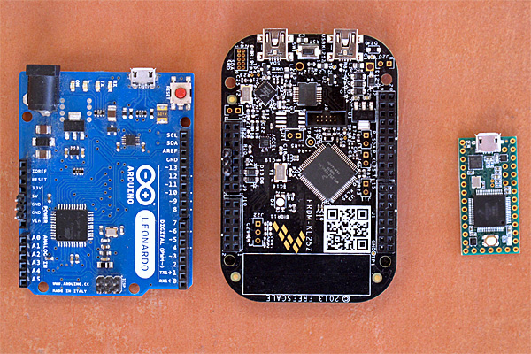
For the past couple of years, I’ve been using the PteroDAQ data acquisition system that my son wrote for the KL25Z board (a second-generation system, replacing the earlier Arduino Data Logger he wrote). He has been working on and off on a multi-platform version of PteroDAQ for over a year, and I finally asked him to hand the project over to me to complete, as I want it much more than he does (he’d prefer to spend his time working on new products for his start-up company, Futuristic Lights).
It has been a while since he worked on the code, and it was inadequately documented, so we’ve been spending some time together just digging into the code to figure out the interfaces, which I’ve been adding comments and docstrings to, so that I can debug the code. Other than the lack of documentation, the code is fairly well written, so figuring out what is going on is not too bad (except in the GUI built using tkinter—like all GUI code, it is a complicated mess, because the APIs for building GUIs are a complicated mess).
The man goal of his multi-platform code was to support Arduino ATMega-based boards and the KL25Z board, while making it relatively easy to add more boards in future. The Arduino code is compiled and downloaded by the standard Arduino IDE, while the KL25Z board code is compiled and downloaded with the MBED online compiler. He has set up the software with appropriate #ifdef checks, so that the same code files can be compiled for either architecture. The knowledge of what features are available on each board and how to request them is stored in one module of the python program that runs on the host computer. As part of the cleaning up, we’ve been moving some of the code around to make sure that all the board-specific stuff is in that file, with a fairly clean interface.
He believed that he had gotten the new version working on the Arduino boards, but not on the KL25Z board. It turned out that was almost true—I got the system working with the Leonardo board (which uses USB communication and has a weird way to get reset) almost immediately, but had to do a number of little bug fixes to get it working with other Arduino boards (which use UART protocol and a different way of resetting). It turned out that the system also worked with the KL25Z after those bug fixes, so he was very close to having it ready to turn over to me.
One of the first things I did was to time how fast the boards would run with the new code—the hope was that the cleaner implementation would have less overhead and so support a higher sampling rate. Initial results on the Arduino boards were good, but quite disappointing on the KL25Z boards, which use a faster processor and so should be able to support much higher speeds. We tracked the problem down to the very high per-packet overhead of the USB packets in the mbed-provided USBSerial code. (He had tried writing his own USB stack for bare-metal ARM, but had never gotten it to work, so we were using the mbed code despite its high overhead.)
There was a simple fix for the speed problem: we stopped sending single-character packets and started using the ability of the MBED code (and the Arduino code for the Leonardo) to send multi-character packets. With this change, we got much better sampling rates (approximate max rate):
| channels |
Leonardo |
Uno/Duemilanove/Redboard |
KL25Z 32x avg |
KL25Z, 1x avg |
| 0 |
13kHz |
4.5kHz |
8.2kHz |
|
| 1 analog |
5kHz |
2.7kHz |
5.5kHz |
8.1kHz |
| 2 analog |
3kHz |
1.9kHz |
3kHz |
8.1kHz |
| 7 digital |
6.5kHz |
3.4kHz |
8.2kHz |
|
It is interesting that the Leonardo (a much slower processor) manages to get a higher data rate than the KL25Z when sending just time stamps. I think that I can get another factor of 3 or 4 speed on the KL25Z by flushing the packets less often, though, so I’ll try that.
By flushing only when needed, I managed to improve the KL25Z performance to
| channels |
KL25Z 32x avg |
KL25Z, 1x avg |
| 0 |
17kHz |
|
| 1 analog |
6.3kHz |
10kHz ?? |
| 2 analog |
3.3kHz |
|
Things get a bit hard to measure above 10kHz, because the board runs successfully for several hundred thousand samples, then I start losing characters and getting bad packets. The failure mode using my son’s faster Linux box is different: we lose full packets when going too fast—which is what PteroDAQ is supposed to do—and the speed at which the failure starts happening is much higher (maybe 23kHz). In other words, what I’m seeing now are the limitations of the Python program on my old MacBook Pro. It does bother me that the Mac seems to be quietly dropping characters when the Python program can’t clear the USB serial input fast enough.
The KL25Z slows down when doing the 32x hardware averaging, because the analog-to-digital conversion is slow—particularly when doing 32× hardware averaging. I think that we’ve currently set things up for a 6MHz ADC clock, with short sampling times, which means that a single-ended 32× 16-bit conversion takes around 134µs and the sampling rate is limited by the conversion times (differential measurements are slower, around 182µs).
There is a problem in the current version of the code, in that interrupts that take longer to service than the interrupt time result in PteroDAQ lying about its sampling rate. I can fix this on the KL25Z by using a separate timer, but the Arduino boards have rather limited timer resources, and we may just have to live with it on them. At least I should add an error flag that indicates when the sampling rate is higher than board can handle.
We had a lot of trouble yesterday with using the bandgap reference to set the voltage levels. It turns out that on the Arduino boards, the bandgap channel is a very high impedance, and it takes many conversion times before the conversion settles to the final value (nominally 1.1V). Switching channels and then reading the bandgap is nearly useless—the MUX has to be left on the bandgap for a long time before reading the value means anything. If you read several bandgap values in quick succession, you can see the values decaying gradually from the value of the previously read channel to the 1.1V reference.
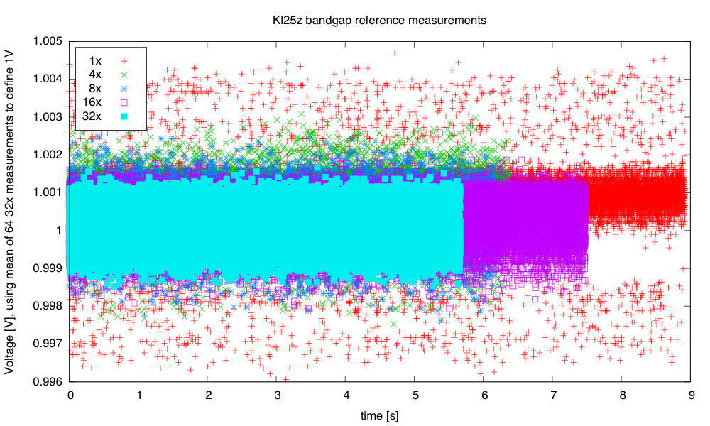
The bandgap on the KL25Z is not such a high-impedance source, but there is some strange behavior when reading it with only 1× averaging—some values seem not to occur and the ds. I recorded several thousand measurements with 1×, 4×, 8×, 16×, and 32× averaging:

The unaveraged (1×) reading seems to be somewhat higher than any of the hardware-averaged ones.
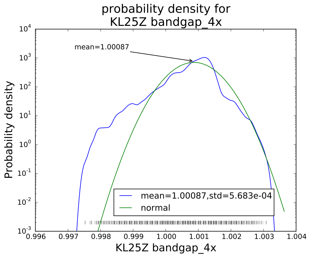
I was curious about how the noise reduced on further averaging, and what the distribution was for each of the averaging levels. I plotted log histograms (using kernel-density estimates of the probability density function: gaussian_kde from the scipy python package) of the PteroDAQ-measured bandgap voltages. The PteroDAQ is not really calibrated—the voltage reference is read 64 times with 32× averaging and the average of those 64 values taken to be 1V, but the data sheet says that the bandgap could be as much as 3% off (that’s better than the 10% error allowed on the ATMega chips).
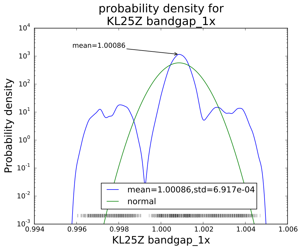
Without averaging, there is a curious pattern of missing values, which may be even more visible in the rug plot at the bottom than in the log histogram.

The smoothed log-histogram doesn’t show the clumping of values that is more visible in the rug plot.
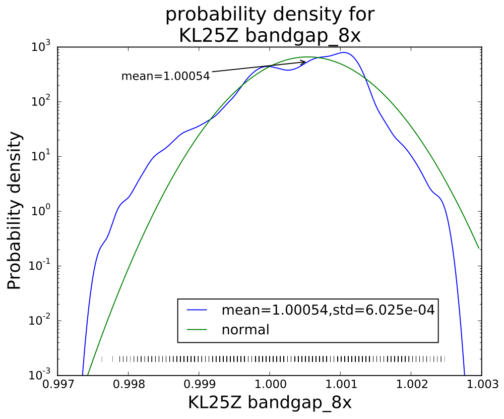
With eight averages, the distribution begins to look normal, but there is still clumping of values.

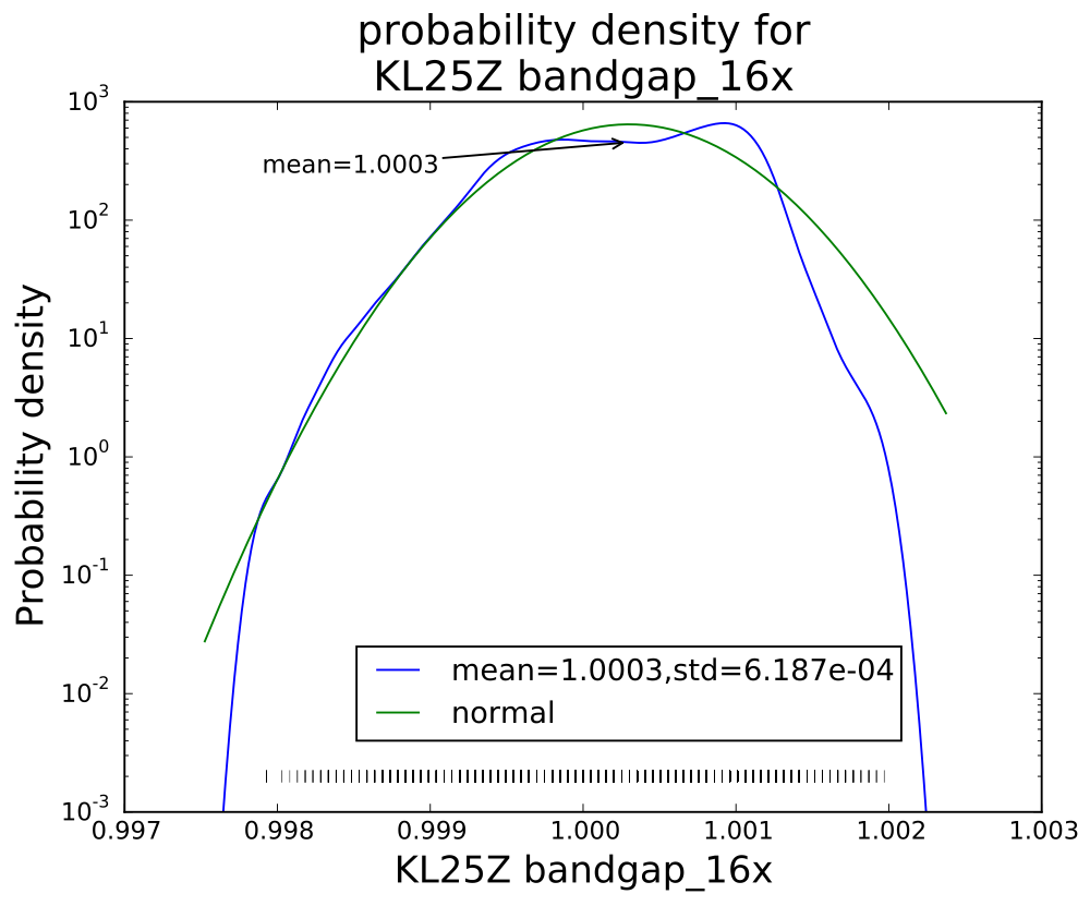
With 16 averages, things look pretty good, but mode is a bit offset from the mean still.

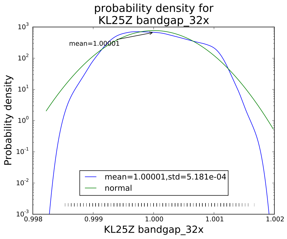
Averaging 32 values seems to have gotten an almost normal distribution.
Interestingly, though the range of values reduces with each successive averaging, the standard deviation does not drop as much as I would have expected (namely, that averaging 32 values would reduce the standard deviation to about 18% the standard deviation of a single value). Actually, I knew ahead of time that I wouldn’t see that much reduction, since the data sheet shows the effective number of bits only increasing by 0.75 bits from 4× t0 32×, while an 8-fold increase in independent reads would be an increase in effective number of bits of 1.5 bits. The problem, of course, is that the hardware averaging is of reads one right after another, in which the noise is pretty highly correlated.
I think that the sweet spot for averaging is the 4× level—almost as clean as 32×, but 8 times faster. More averaging improves the shape of the distribution a little, but doesn’t reduce the standard deviation by very much. Of course, if one has a low-frequency signal with high-frequency noise, then heavier averaging might be worthwhile, but it would probably be better to sample faster with the 4× hardware averaging, and use a digital filter to remove the higher frequencies.
The weird distribution of values for the single read is not a property of the bandgap reference, but of the converter. I made a voltage divider with a couple of resistors to get a voltage that was a fixed ratio of the supply voltage (so should give a constant reading), and saw a similar weird distribution of values:
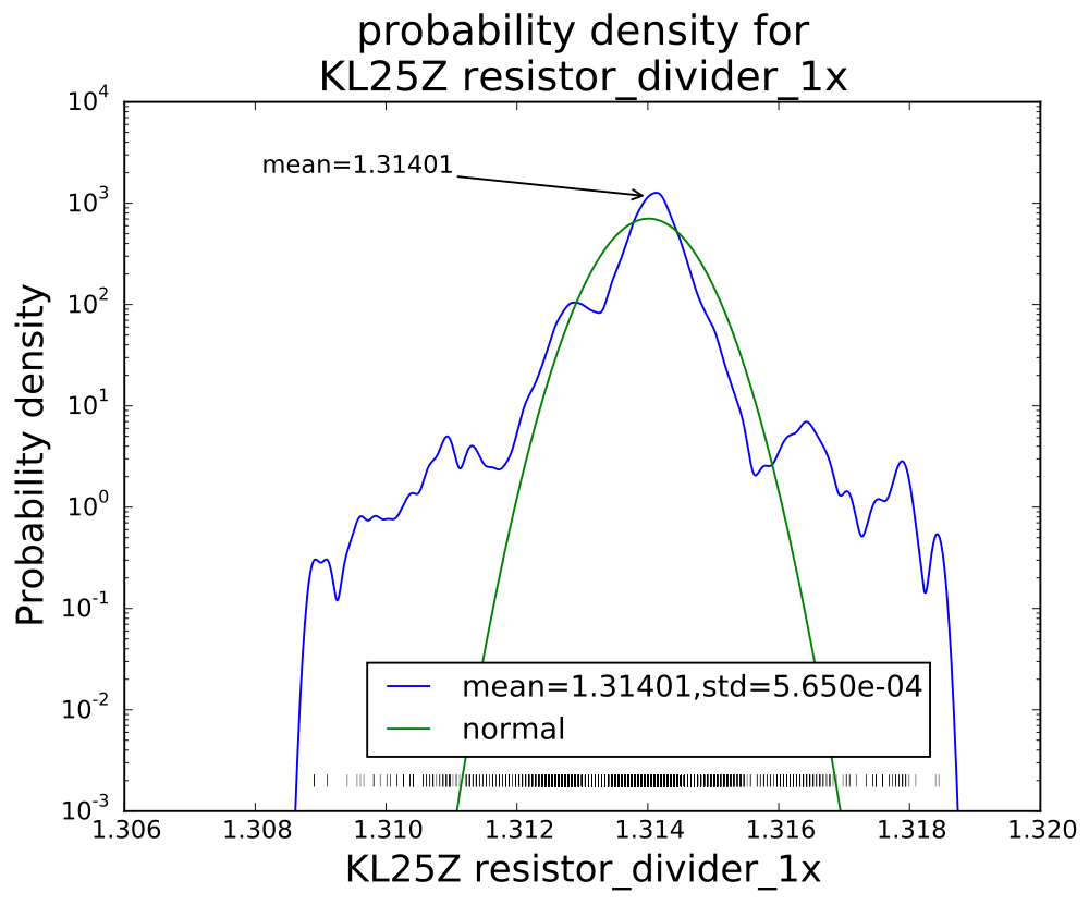
The distribution of single reads is far from a normal noise distribution, with fat tails on the distribution and clumping of values.
With 32× sampling, the mean is 1.31556 and the standard deviation 5.038E-04, with an excellent fit to a Gaussian distribution.
Filed under:
Circuits course,
Data acquisition Tagged:
Arduino,
histograms,
KL25Z,
noise,
PteroDAQ,
sampling frequency 


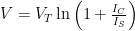 , where IS is the saturation current of the diode, using the following setup


 , where IS is the saturation current of the diode, using the following setup


