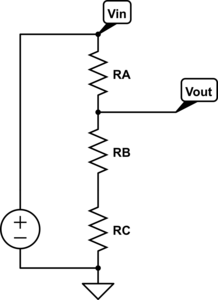
In More on automatic measurement of conductivity of saline solution, I suggested using a simple voltage divider and a microcontroller to make conductivity measurements with polarizable electrodes:
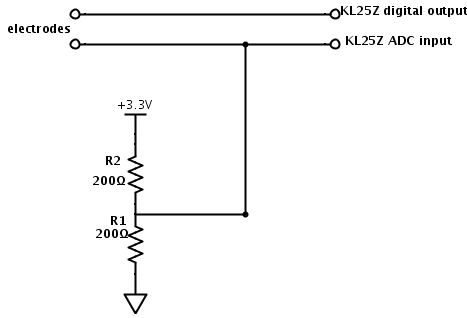
Simplified circuit for conductivity tester.
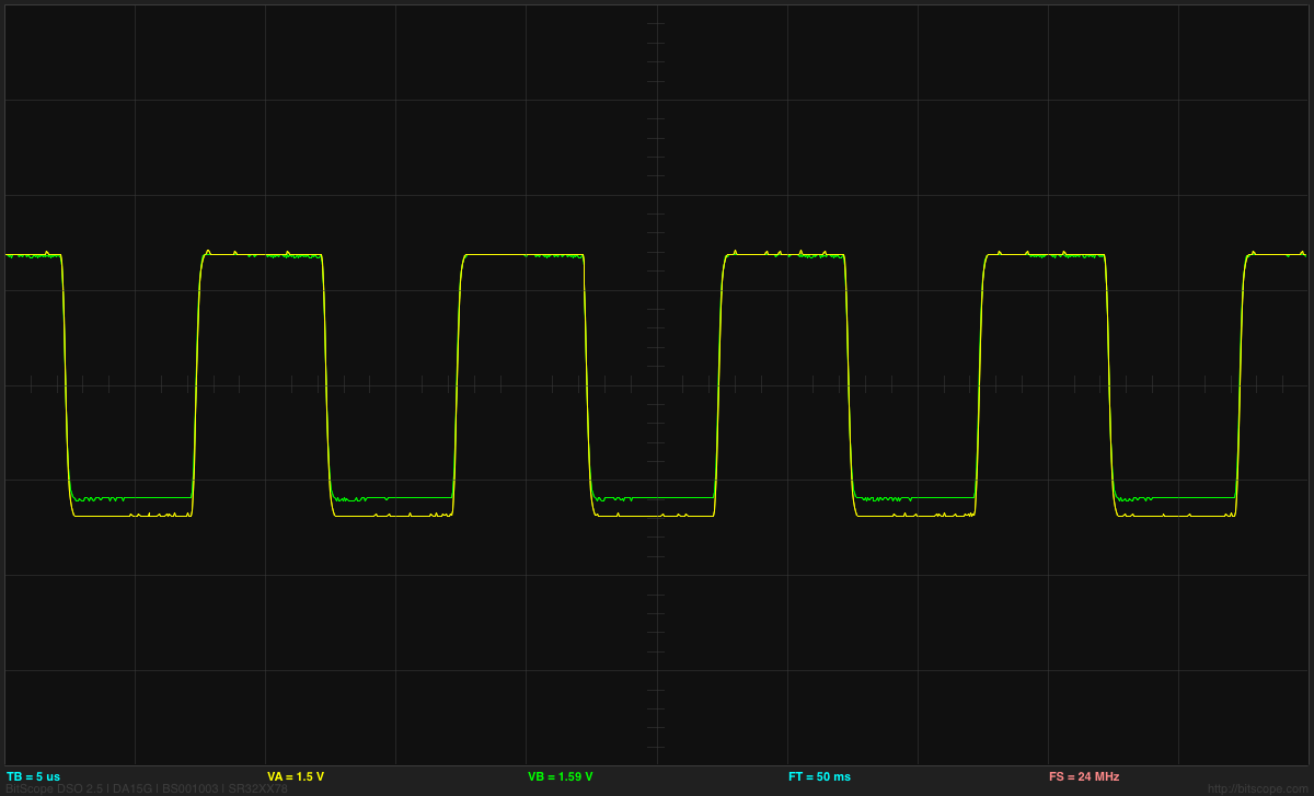
I found that putting in a 100kHz square wave worked well:
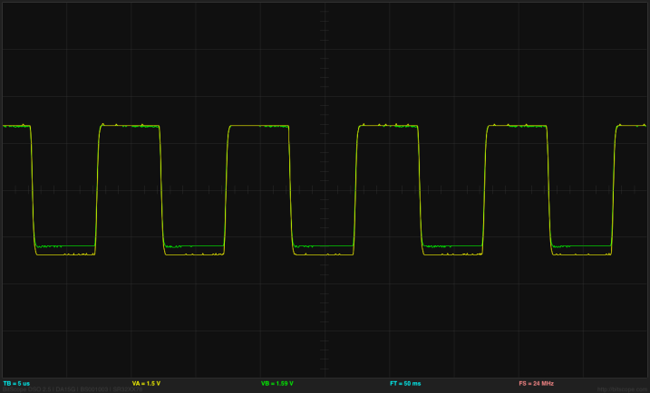
At 100kHz, both the voltage waveforms (input and output) look like pretty good square waves.
I have not yet figured out a good way on the KL25Z to provide the 100kHz signal, sample the outputs at fixed points, and communicate the result out the USB port. Using PWM for the output was handy for just generating the output (once I fixed mbed’s off-by-one bug in their pwmout_api.c file), but that makes connecting up the analog reads more difficult. I think that I may be better off not using PWM, but using a timer interrupt to read the analog value, change the output, and do the subtraction. It would be fairly easy to arrange that (though I’ll probably have to figure out all the registers for the sample-and-hold and the analog-to-digital converter, as the mbed AnalogIn routine is unlikely to have the settings I want to use). The hard part remains the interface to the host computer, as mbed does not include a simple serial interface and serial monitor like the Arduino IDE. [Correction 2013 Dec 25: my son points out that the mbed development kit has a perfectly usable serial USB interface—I had overlooked the inheritance from "Stream", which has all the functions I thought were missing. I should be able to use the Arduino serial monitor with the Freedom KL25Z board, as long as the serial interface is set up right.]
Because I’m more familiar with the Arduino environment, and because I already have Arduino Data Logger code for the host end of the interface, I started by making a simple loop that toggles the output and reads the value after each change in output. After repeating this several times (40 or 100), I take the last difference as the output and report that to the data logger. I couldn’t get the frequency up where I really want it (100kHz), because the Arduino analog-to-digital converter is slow, but I was able to run at about 4kHz, which would be adequate.
Because there needs to be time for the serial communication, I did bursts of pulses with pauses between bursts. The bursts were alternating as fast as the analog inputs were read for a fixed number of cycles, and the start of the bursts was controlled by the Arduino data logger software. Although the ends of the bursts looked the same on the oscilloscope, with the same peak-to-peak voltage, I got different readings from the Arduino depending on the spacing between the bursts. I’m not sure what is causing the discrepancy.
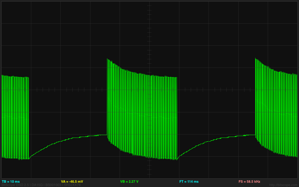
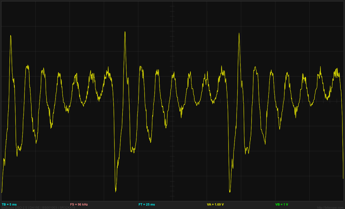
A difference at the beginnings of the bursts I would understand as the space between the bursts put a DC voltage across the electrodes which gradually charged them up, so that the first few pulses actually end up going outside the range of the ADC:
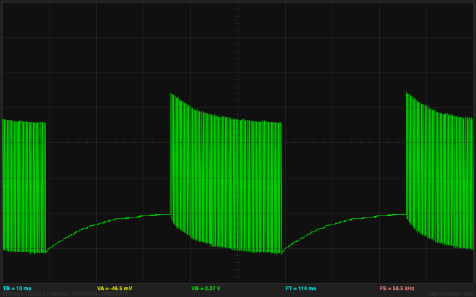
The bottom of the grid is 0v, and the first pulse goes up to 5.442v. The pulses are at about 4kHz, but the bursts start 50msec apart.
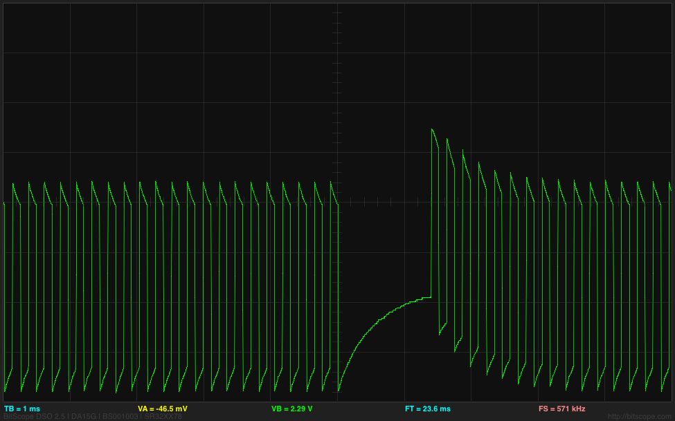
The differences at the ends of the bursts as I change the spacing between bursts are probably also due to the charging, though I don’t see that clearly on the oscilloscope. I really don’t like the idea of having a DC bias across the electrodes, as we get electrolysis, with hydrogen bubbles forming on the more negative electrode. No oxygen bubbles form, probably because any oxygen released is reacting with the stainless steel to form metal oxides. If I increase the voltage and current, I get a lot of hydrogen bubbles on the negative electrode, some rusty looking precipitate coming off the positive electrode (probably an iron oxide), and a white coating building up on the positive electrode (probably a chromium oxide).
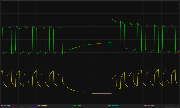
By putting a 4.7µF capacitor between the Arduino output and the electrode, I can reduce DC bias on the electrodes and get a more consistent signal from the Arduino, almost independent of the spacing between the bursts:

By using a 25msec spacing between the beginnings of bursts, I can get both the end of the burst and the beginning of the burst on the oscilloscope at once.
Using a 4.7µF capacitor between the square wave output and the electrodes results in sharp peaks across the resistor, but a more consistent reading from the Arduino ADC.
The voltage across the electrodes still does not average to 0v, as the pair of resistors provides a bias voltage halfway between the rails, but the pulse does not really swing rail to rail, but from 0.28v to 4.28v. I think that the low-pass filter for setting the bias voltage that I suggested in More on automatic measurement of conductivity of saline solution may be a good idea after all, to make sure that there is no residual DC bias.
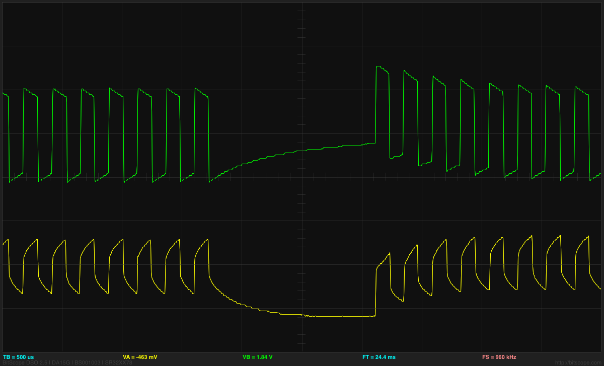
I can use the differential inputs of the Bitscope DP01 to look at the voltage across the electrodes and across the resistor to get voltage and current traces for the electrodes:
The central horizontal line is 0V for both traces here. The green trace is the voltage at the undriven electrode (@ 2v/division) and so corresponds to the current, and the yellow trace is the voltage between the electrodes (@0.2v/division).
Note that the voltage on the undriven electrode does run a little below 0V, outside the range of the Arduino ADC. The voltage ratio of 0.248v/4.16v, together with the 100Ω Thévenin equivalent resistance results in a 5.47Ω resistance between the electrodes. (Note: this is no longer a 1M NaCl solution—there has been evaporation, plus contamination from iron oxides, and the electrodes are not covered to the depth defined by the plastic spacer.)
I don’t know whether the conductivity meter is a good project for the freshman design seminar or not—I don’t expect the students to have the circuit skills or the programming skills to be able to do a design like this without a lot of coaching. Even figuring out that they need to eliminate DC bias to eliminate electrolysis may be too much for them, though I do expect all to have had at least high-school chemistry. It is probably worth doing a demo of putting a large current through electrodes in salt solution, to show both the hydrogen bubbles and the formation of the oxides. I could probably coach freshmen through the design, if they were interested in doing it, so I’ll leave it on the feasible list.
The square-wave analysis is not really suitable for a circuits course, so I think I’ll stick with sine-wave excitation for that course.
Filed under:
Circuits course,
freshman design seminar Tagged:
Arduino,
bioengineering,
circuits,
conductivity,
electrodes,
KL25Z,
voltage divider 


 You can get a lot of quick info from a business card — name, job title, contact info — and now you can also see your heart beat.