Posts with «voltage divider» label

Wheel of Resistors Form Unique Rotary Encoder

Continuing his tradition of making bits of wire and scraps of wood work wonders, [HomoFaciens] is back with a unique and clever design for an electromechanical encoder.

There are lots of ways to build an encoder, and this is one we haven’t seen before. Not intended in any way to be a practical engineered solution, [HomoFaciens]’ build log and the video below document his approach. Using a rotating disc divided into segments by three, six or eight resistors, the encoder works by adding each resistor into a voltage divider as the disc is turned. An Arduino reads the output of the voltage divider and determines the direction of rotation by comparing the sequence of voltages. More resistors mean higher resolution but decreased maximum shaft speed due to the software debouncing of the wiped contacts. [HomoFaciens] has covered ground like this before with his tutorial on optical encoders, but this is a new twist – sort of a low-resolution continuous-rotation potentiometer. It’s a simple concept, a good review of voltage dividers, and a unique way to sense shaft rotation.

Is this all really basic stuff? Yep. Is it practical in any way? Probably not, although we’ll lay odds that these encoders find their way into a future [HomoFaciens] CNC build. Is it a well-executed, neat idea? Oh yeah.


Filed under: misc hacks

Still more on automatic measurement of conductivity of saline solution

In More on automatic measurement of conductivity of saline solution, I suggested using a simple voltage divider and a microcontroller to make conductivity measurements with polarizable electrodes:

Simplified circuit for conductivity tester.

I found that putting in a 100kHz square wave worked well:

At 100kHz, both the voltage waveforms (input and output) look like pretty good square waves.

I have not yet figured out a good way on the KL25Z to provide the 100kHz signal, sample the outputs at fixed points, and communicate the result out the USB port.  Using PWM for the output was handy for just generating the output (once I fixed mbed’s off-by-one bug in their pwmout_api.c file), but that makes connecting up the analog reads more difficult.  I think that I may be better off not using PWM, but using a timer interrupt to read the analog value, change the output, and do the subtraction.  It would be fairly easy to arrange that (though I’ll probably have to figure out all the registers for the sample-and-hold and the analog-to-digital converter, as the mbed AnalogIn routine is unlikely to have the settings I want to use).   The hard part remains the interface to the host computer, as mbed does not include a simple serial interface and serial monitor like the Arduino IDE. [Correction 2013 Dec 25: my son points out that the mbed development kit has a perfectly usable serial USB interface—I had overlooked the inheritance from "Stream", which has all the functions I thought were missing. I should be able to use the Arduino serial monitor with the Freedom KL25Z board, as long as the serial interface is set up right.]

Because I’m more familiar with the Arduino environment, and because I already have Arduino Data Logger code for the host end of the interface, I started by making a simple loop that toggles the output and reads the value after each change in output.  After repeating this several times (40 or 100), I take the last difference as the output and report that to the data logger.  I couldn’t get the frequency up where I really want it (100kHz), because the Arduino analog-to-digital converter is slow, but I was able to run at about 4kHz, which would be adequate.

Because there needs to be time for the serial communication, I did bursts of pulses with pauses between bursts.  The bursts were alternating as fast as the analog inputs were read for a fixed number of cycles, and the start of the bursts was controlled by the Arduino data logger software. Although the ends of the bursts looked the same on the oscilloscope, with the same peak-to-peak voltage, I got different readings from the Arduino depending on the spacing between the bursts. I’m not sure what is causing the discrepancy.

A difference at the beginnings of the bursts I would understand as the space between the bursts put a DC voltage across the electrodes which gradually charged them up, so that the first few pulses actually end up going outside the range of the ADC:

The bottom of the grid is 0v, and the first pulse goes up to 5.442v. The pulses are at about 4kHz, but the bursts start 50msec apart.

The differences at the ends of the bursts as I change the spacing between bursts are probably also due to the charging, though I don’t see that clearly on the oscilloscope. I really don’t like the idea of having a DC bias across the electrodes, as we get electrolysis, with hydrogen bubbles forming on the more negative electrode. No oxygen bubbles form, probably because any oxygen released is reacting with the stainless steel to form metal oxides. If I increase the voltage and current, I get a lot of hydrogen bubbles on the negative electrode, some rusty looking precipitate coming off the positive electrode (probably an iron oxide), and a white coating building up on the positive electrode (probably a chromium oxide).

By putting a 4.7µF capacitor between the Arduino output and the electrode, I can reduce DC bias on the electrodes and get a more consistent signal from the Arduino, almost independent of the spacing between the bursts:

By using a 25msec spacing between the beginnings of bursts, I can get both the end of the burst and the beginning of the burst on the oscilloscope at once.
Using a 4.7µF capacitor between the square wave output and the electrodes results in sharp peaks across the resistor, but a more consistent reading from the Arduino ADC.

The voltage across the electrodes still does not average to 0v, as the pair of resistors provides a bias voltage halfway between the rails, but the pulse does not really swing rail to rail, but from 0.28v to 4.28v.  I think that the low-pass filter for setting the bias voltage that I suggested in More on automatic measurement of conductivity of saline solution may be a good idea after all, to make sure that there is no residual DC bias.

I can use the differential inputs of the Bitscope DP01 to look at the voltage across the electrodes and across the resistor to get voltage and current traces for the electrodes:

The central horizontal line is 0V for both traces here. The green trace is the voltage at the undriven electrode (@ 2v/division) and so corresponds to the current, and the yellow trace is the voltage between the electrodes (@0.2v/division).

Note that the voltage on the undriven electrode does run a little below 0V, outside the range of the Arduino ADC.  The voltage ratio of 0.248v/4.16v, together with the 100Ω Thévenin equivalent resistance results in a 5.47Ω resistance between the electrodes.  (Note: this is no longer a 1M NaCl solution—there has been evaporation, plus contamination from iron oxides, and the electrodes are not covered to the depth defined by the plastic spacer.)

I don’t know whether the conductivity meter is a good project for the freshman design seminar or not—I don’t expect the students to have the circuit skills or the programming skills to be able to do a design like this without a lot of coaching.  Even figuring out that they need to eliminate DC bias to eliminate electrolysis may be too much for them, though I do expect all to have had at least high-school chemistry. It is probably worth doing a demo of putting a large current through electrodes in salt solution, to show both the hydrogen bubbles and the formation of the oxides.  I could probably coach freshmen through the design, if they were interested in doing it, so I’ll leave it on the feasible list.

The square-wave analysis is not really suitable for a circuits course, so I think I’ll stick with sine-wave excitation for that course.


Filed under: Circuits course, freshman design seminar Tagged: Arduino, bioengineering, circuits, conductivity, electrodes, KL25Z, voltage divider

Fifth day of circuits class

I feel pretty good about today’s lecture, though things got a little rushed at the end.

Three-resistor voltage divider for the first question.

I started with a “do now” question, similar to the one from Monday. Actually, I started with 2 questions. The first just asked what the output voltage would be for a 3-resistor voltage divider. The second repeated the question from Monday, but with the additional constraint that the power supply was 5 volts:

You have sensor whose resistance varies from 1kΩ to 4kΩ with the property it measures and a 5v power supply.  Design a circuit whose output voltage varies from 1v (at 1kΩ) to 2v (at 4kΩ).

Several students realized that the first question was a hint for the second one and that the variable resistor had to be RB or RC, and could set up the equations and solve for RA and RC.  This is a better performance than on Monday’s “do now”, but only about 1/3 of the class got it completely, and several of them were not confident of their results, so we again took time to go over the whole solution. I think that everyone (or almost everyone) understood the design process and how to set up and solve the equations by the end of the presentation, which I drew out of the students as much as possible.  I also mentioned that we could have solved the problem with a different circuit (putting RC in parallel with RB instead of in series), but did not further elaborate on that point.

The do-now plus going over the solution took about 33 minutes, which is a little more time than I’d like to be spending on these questions.  It would be good to get the time down to 15 minutes, but I don’t see how to do that without losing half the class.  If the problems are easy enough that everyone gets them, then there is no point to taking up any class time with them, and if they are hard enough that 1/3 to 2/3 of the class don’t get them, then they need to be gone over in class.

After the do-now, we spent a little time discussing the “fit” command of gnuplot, since the students have to fit models to the data they collect tomorrow, and I’m not providing them a script this time (though they can modify the script that was provided in the first lab).

Finally, we got to the theoretical meat of the class—we discussed what sound was (ending up with variations in pressure for a fluid, though we discussed briefly transverse and shear waves in solids).  Then I introduced microphones as transducers, trying to get the students to remember their elementary mechanics, so that we could do pressure→force→displacement→1/capacitance→voltage for electret mics.  The hardest part was getting students to remember that a spring-mounted object had force proportional to displacement (a lot remembered the energy was somehow related to displacement squared and got stuck on that formula).  I suspect that the local physics department would not be seeing a high score on the Force Concept Inventory for students coming out of their physics classes, as a lot of them seem to have concentrated on cramming formulas rather than learning fundamental concepts.  Someone did remember Q=CV and someone else could reason from wanting voltage proportional to displacement to needing constant charge which let me introduce both conventional capacitance microphone (with a large resistor to voltage source) and electrets.  I also explained that the electret had an enormous resistance, so we couldn’t get any measurable current out of it, and we needed an FET transistor to convert the voltage to a current.

Because both the do-now and extracting vague memories of physics from the students took longer than I had planned, we were a bit rushed for the last part of the lesson, which was a simple model of Ids vs Vds for the FET output stage of the electret mic. I asked for advice on drawing the plots for resistors and for current sources, and got the appropriate straight lines.  I then drew a smooth transition between them and claimed that the simple FET models usually consisted of a linear region at low voltage (which my co-instructor refers to as the “triode” region, a usage I’ve seen in some other presentations) and a saturation region at high voltage, and that we usually try to stay out of the sublinear region in between.

I also said that the saturation region is not really constant, but has a slight upward slope, since they will be measuring the I-vs-V characteristic of the electret microphones tomorrow, and they will certainly be observing that.  The lab handout gives them 4 models to fit: linear, constant current, an empirical blend of the two, and a model that allows current increase in the saturation region.  Neither the 3rd nor the 4th model match the ones usually used in circuit simulators, but I had trouble fitting parameters to those models, even with voltage-modulated channel lengths, so I gave up and produced simple models with few parameters that can be fit pretty easily. We’ll be revisiting FETs again before the power-amp lab (where they’ll use pMOS and nMOS power FETs to make a class-D amplifier). Somewhere around then, I’ll have to give them some usable models for how saturation current varies with gate voltage, which I deliberately did not cover in this lecture.

I’m a bit worried about how big tomorrow’s lab is.  There are again 2 parts:

  • the DC characterization of the mic using the Arduino to gather data (plus a few hand-collected points for higher voltages than we can subject the Arduino to)
  • designing a pull-up resistor to bias the mic into its normal operating range (in the saturation region) and observing the microphone output on the oscilloscope.  I also asked students to hook up their loudspeakers to the signal generators, to provide known inputs to the mic, and some other little stuff, but I’ll probably be happy if everyone gets the first part done and manages to observe waveforms on the scope.

On Friday, most of the lecture will be standard EE stuff by my co-instructor (probably current sources, Thévenin equivalents, and Norton equivalents).  I may have a do-now question at the beginning of the class, if I can come up with one that I think is pedagogically useful.


Filed under: Circuits course Tagged: Arduino, circuits, course design, electret microphone, teaching, voltage divider

Fourth day of circuits class

Today’s class went much better than last Friday’s.

I took the advice one of the students gave me last we and started with a “do now” question.  (She had actually suggested an “exit ticket”, but I don’t have the time management skills to leave a block of time at the end of class.)  The question I asked was a design task that was easy if you knew what you were doing, but subtly harder than the standard sort of text-book question, because it was a design question, not an analysis question:

You have sensor whose resistance varies from 1kΩ to 4kΩ with the property it measures.  Design a circuit whose output voltage varies from 1v (at 1kΩ) to 2v (at 4kΩ).

I gave the students 10 minutes to work on this at the beginning of class.  A good question to prompt discussion (according to the peer instruction blogs and websites) should be answerable by 30–80% of the students.  More than that and the question was too easy to be useful, and less than that and the question is too hard for peer discussion to be worthwhile.  It turned out that no one had gotten it after 10 minutes (too hard to use as a peer instruction question), so we used it as the basis for a class discussion.

Almost everyone realized that the desired circuit was a voltage source and a voltage divider (not too surprising, since that’s the only circuit they’ve used so far).  The majority also realized that the variable resistor had to be on the lower leg, between the output and ground, and a couple of the students could articulate why.  I suggested the common heuristic of trying extreme values (0 and ∞) for the variable resistor, to see whether the output voltage would go up or down as the resistance changed.

The students were then able to set up the simultaneous equations to solve for the input voltage and the fixed resistance.  The hole in everyone’s thinking when working on the problem initially is that they had not considered the voltage of the source as a design parameter to solve for, though one student had asked about it. This was the blind spot I was expecting, so I was able to use it as a teachable moment.  After we had the equations set up using mainly student input, I gave the students another minute or two to solve them, and about half the class was able to solve them correctly in the time provided. (I suspect that everyone could have if given enough time, but I didn’t want to take any more time in class—those who didn’t solve it in class could practice their algebra at home if they needed to.)  One student had made an algebra or arithmetic mistake, and gotten a source voltage smaller than one of the desired output voltages.  This was also a good mistake to get, since we could use it to talk about sanity checks on results.

I think that the 20 or so minutes of class was well spent, as we uncovered several important misconceptions, and raised awareness of all unspecified variables as potential design parameters, reasoning using extreme values, and the usefulness of sanity checks.

After that, we spent some time discussing different temperature sensors.  From the students, I got thermistor, infrared thermometer, mercury thermometer+camera, and enzyme + other sensor (pH, conductivity, color, …). I added RTD, silicon band-gap, and thermocouple to the mix.  We talked a little about the advantages and disadvantages of each. At the end, I also threw in bimetallic strips and tilt switches for one-bit digitization of temperature.  I wonder how many students will look at the thermostats in their apartments and try to figure out what sensor they include.

For the remainder of the class, we talked about gnuplot commands, particularly the “plot” command.

After class, several of us went over to the lab, where my son met us and helped the students install the DataLoger, python, pyserial, the Arduino environment, and gnuplot.  While he was doing that, I borrowed an Uno R3 Arduino board and made sure that all the computers in the labs had the drivers installed for it.  We had 2 installation failures: on one Windows laptop, my son was unable to get the serial ports to work and one Mac laptop couldn’t install gnuplot.

The problem with the gnuplot installation on that Mac was not solvable by the techniques in the comments for Installing gnuplot—a nightmare, because all the methods there assume that you can install the command-line tools “make” and “gcc”.  The Mac had 10.6.8 installed, but the student had never bothered to install the development tools and had lost the original CD-ROM with the Xcode tools on it.  The Apple Developer site does not provide the command-line tools for anything older than 10.7.3.  The only workaround we could find was to download the 4.1GByte complete Xcode suite for OS 10.6.8, which I was not willing to wait around for. (Other students with 10.6.8 had no trouble installing gnuplot, because they already had the command-line tools, though they’d never used them.)

I did not look at the problem on the Windows machine (the student had to leave for class before I became available), but I don’t know that I could have done anything—my son knows more about Windows than I do, so if he was stuck, I probably would have been also.

Next year I’m going to want to do an install session before the first lab.  (Or, if we go to 2 labs a week, as the first lab.)

On Wednesday, I’ll start with another “do now” question, though I’m not sure what it’ll be on, since I’ve not yet gotten to the material for this week’s lab: how a microphone works. I’ll do a tiny bit of gnuplot (just the “fit” command) and try to get through how a microphone works and an idealized i-vs-v plot for the FET output of the microphone.


Filed under: Circuits course Tagged: Arduino, circuits, gnuplot, parts, teaching, temperature measurement, voltage divider

Temperature lab, part 3: voltage divider

In Temperature lab, part2, I carefully measured the resistance vs. temperature curve for the Vishay BC Components NTCLE413E2103F520L thermistor, finding that either my thermometer was badly miscalibrated, or the manufacturer’s data sheet was misleading.  I got a resistance of 9.7kΩ (not 10kΩ±1%) at 25° C and a B-value of 3174°K, not 3435°K±1%.  A big part of the discrepancy is that I calibrated over a different temperature range, and the measured values deviated most from the manufacturer’s spec at low temperatures.

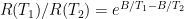
Actually, the manufacturer’s data sheet is not as bad as all that.  They give specs for the ratio of the resistance at various temperatures to the resistance at 25° C, and their numbers do not fall along a simple curve.  The report the B-value as a 2-point fit for T=25° C and T=85° C, but they also report resistance values every 5° C from –40° C to 105° C.  One can compute the B-value for any pair:

But even if I use their calibration data down to 0° C, I don’t get as small a B-value as I get from my measurements. My calibration curve does not fit their spec, even if I look at the table, rather than the simple B-value model (though the table is closer to my measurements, it doesn’t match).

How big a difference would if make if I used their curve rather than mine?  At R=6685Ω, we get the same temperature either way (96.446° F).  At the resistance they claim for 0° C (27348Ω), their B-value model would give 33.90° F and mine would give 29.37° F.  At the resistance I measured for 0° C (25.5kΩ), their model would give 36.67° F, while mine gives 32.32° F (which is closer than the measurement error I had on temperatures).  So it looks like relying blindly on their B-value model introduces an error of over 4° F at low temperature, but in a digital thermometer for human body temperature, one would get nearly the same result with either calibration.

Voltage divider

The second part of the lab was to use the calibration curve to design a circuit to convert the resistance variation into a voltage variation that is nearly linear with temperature, at least over a small range.  The simplest circuit to convert a resistance to a voltage is a voltage divider, which just requires a voltage source and another resistor.

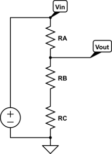
A simple voltage divider for converting the thermistor resistance to a voltage. Because I want the output voltage to increase with temperature, but the resistance R(T) decreases with temperature, I put the thermistor on the top branch and fixed resistance on the lower branch.
Circuit drawn with the Circuit Lab editor.

The formula for the output voltage is simple: , where we are approximating for temperature T in Kelvin. We’d like the voltage to be as linear as possible, which means we want the second derivative of Vout with respect to T to be zero. Obviously, we can’t do that for all values of T, but we might be able to do it for a particular value of T, and to have a small second derivative in that neighborhood.

We can take the derivatives by hand (or use a tool like Maple or Mathematica):


The second derivative is 0 if , that is if .

We can use this formula to set the value for any temperature, for example, if we want linearity around 98.6° F (310.15° K), we can set the series resistor to 4323.64Ω.

Expected voltage curve using a voltage divider with series resistor optimized for 98.6° F. Note that the curve is fairly linear from about 70° F to about 130° F (where the red non-linear curve and the green linear approximation at 98.6° F are quite close.

Of course, commercially available resistors don’t come in values like 4323.64Ω, so in doing a design one has to pick an available resistor, using the EIA table of standard resistor values.  A 4.7kΩ resistor looks pretty close, which would be color code yellow-violet-red.  Too bad that I don’t have one.  I do have a 5.1kΩ resistor, which would be optimal for linearizing at 90.06° F.  We should, of course, ask students to do the resistor selection for a different temperature than the one we use in an example, and they should be using their own B-value.

Testing the voltage divider

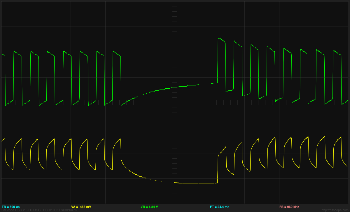
I set up the voltage divider on a breadboard.  Because I knew my wall wart had a huge ripple, I added a low-pass RC filter consisting of a 100Ω resistor and a 470µF electrolytic capacitor.  This slightly complicates the analysis of the voltage output, since the Vdd voltage is itself dependent on a voltage divider.

Low-pass filter to clean up the output of the wall wart. With the low-pass filter in place, we can model the power supply as a 5.166V source and 100Ω series resistor.

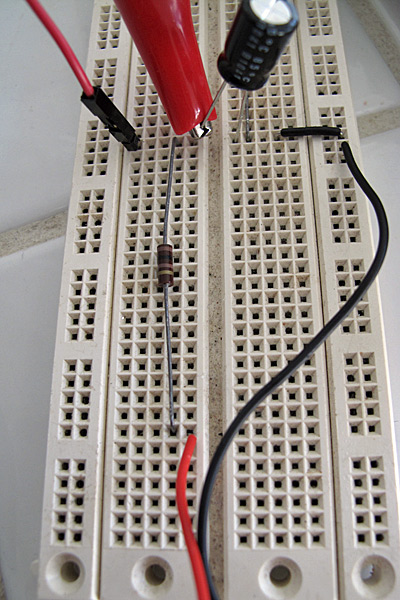
Here is what the low-pass filter looks like on the breadboard. The red and black wires from the bottom come from the connector to the wall wart. The 100Ω resistor runs vertically up the center, and the electrolytic capacitor connects across to the ground. The red clip lead is from the multimeter and is set up for measuring the voltage at the output of the filter.

Here is the full breadboard, showing the RC filter, the series resistor, the leads to the thermistor (the red and yellow lines with the crimp-on connectors), and the clip leads to the multimeter (the red and black alligator clips). I’ve found it very handy to have a number of double-sided header pins to make easy connection points on the breadboard for clip leads.

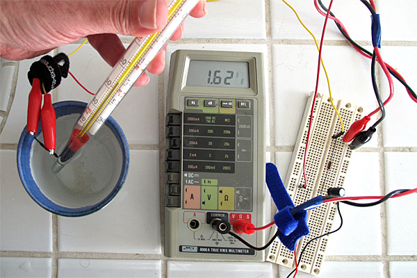
Here is the setup used for testing. The thermistor and thermometer are in the ceramic-cup water bath, with the thermometer held to keep the bulb in contact with the thermistor. You can see that the least-significant digit of the LCD display is a bit hard to read—applying some pressure to the display often makes it readable. Clip leads are essential to doing this experiment—holding the multimeter probes to test points would be a major hassle.

I only made 21 measurements of voltage, since I was not going to be fitting a model to the data, but just using the model I fit from the resistance measurements.

Plot of measured and theoretical voltage vs. temperature for the thermistor. The non-linear theoretical curve seems to be a pretty good fit (though it was not fit on this data, but on the previous series of resistance measurements).

The range of the voltages with the series resistor (from about 0.85v at freezing to 4.15v at boiling) is fairly reasonable for direct conversion to digital for the Arduino 10-bit ADC. In the middle of the range, the slope is about 0.0233 V/°F, which would give a resolution of about 0.2°F for Arduino readings.  (Of course, with the Arduino, we would not need the low-pass filter, and Vdd would be a well-regulated 5v, so this calibration curve would have to be redone.)  Even if we use the computational power of the Arduino to correct the non-linearity of the voltage curve, it is still useful to select the series resistor for the temperature we are most interested in, since that point gets the largest slope and hence the highest temperature resolution for fixed-size steps in voltage quantization.

Series-parallel

A lot of thermistor circuits on the web have a resistor in parallel with the thermistor, as well as the one in series. I wondered what the effect of this extra resistor was.

Circuit with resistor in parallel with the thermistor, as well as in series.

I tried analyzing this circuit also, using the same brute-force approach of computing the second derivative of the voltage and setting it to zero.  I got a result that surprised me initially:  the second derivative is zero if , where is the resistance one would get for putting the series and parallel resistors in parallel. This is exactly the same condition as before, but with replacing the series resistor .

After I thought about this for a while, I realized that I should have been able to get there directly. If you think of the circuit as connecting the thermistor to a voltage divider consisting of R2 and R1, then you can replace the ground and that voltage divider by the Thévenin equivalent, which would be a voltage source with voltage and a series resistor consisting of  R1 and R2 in parallel: .  The only reason to put in a parallel resistor would be to restrict the voltage range (which might be useful if the output were to be amplified, but is not useful if the output is going directly into an analog-to-digital converter whose full-scale range is 0 to Vdd).


Filed under: Circuits course Tagged: Arduino, bioengineering, circuits, course design, teaching, temperature measurement, Thévenin equivalent, thermistor, voltage divider