At Arduino Day, I talked about a project I and my collaborators have been working on to bring machine learning to the maker community. Machine learning is a technique for teaching software to recognize patterns using data, e.g. for recognizing spam emails or recommending related products. Our ESP (Example-based Sensor Predictions) software recognizes patterns in real-time sensor data, like gestures made with an accelerometer or sounds recorded by a microphone. The machine learning algorithms that power this pattern recognition are specified in Arduino-like code, while the recording and tuning of example sensor data is done in an interactive graphical interface. We’re working on building up a library of code examples for different applications so that Arduino users can easily apply machine learning to a broad range of problems.

The project is a part of my research at the University of California, Berkeley and is being done in collaboration with Ben Zhang, Audrey Leung, and my advisor Björn Hartmann. We’re building on the Gesture Recognition Toolkit (GRT) and openFrameworks. The software is still rough (and Mac only for now) but we’d welcome your feedback. Installations instructions are on our GitHub project page. Please report issues on GitHub.

Our project is part of a broader wave of projects aimed at helping electronics hobbyists make more sophisticated use of sensors in their interactive projects. Also building on the GRT is ml-lib, a machine learning toolkit for Max and Pure Data. Another project in a similar vein is the Wekinator, which is featured in a free online course on machine learning for musicians and artists. Rebecca Fiebrink, the creator of Wekinator, recently participated in a panel on machine learning in the arts and taught a workshop (with Phoenix Perry) at Resonate ’16. For non-real time applications, many people use scikit-learn, a set of Python tools. There’s also a wide range of related research from the academic community, which we survey on our project wiki.

For a high-level overview, check out this visual introduction to machine learning. For a thorough introduction, there are courses on machine learning from coursera and from udacity, among others. If you’re interested in a more arts- and design-focused approach, check out alt-AI, happening in NYC next month.

If you’d like to start experimenting with machine learning and sensors, an excellent place to get started is the built-in accelerometer and gyroscope on the Arduino or Genuino 101. With our ESP system, you can use these sensors to detect gestures and incorporate them into your interactive projects!

Yesterday, my son was thinking of adding a microphone to the design he is working on, and was considering adding a fast Fourier transform (FFT) to detect pitch.

He spent a few hours after his 10 a.m.–5 p.m. theater class reading about the FFT algorithm. He found an implementation of the FFT for an Arduino, which he tried reading along with the FFT explanations he found on the web.  I’m actually surprised the the Arduino was capable of doing an FFT, given the slowness of the processor.  It is true that the example code only does a 64-sample FFT with a sampling rate of 1kHz, using 8-bit samples and 16-bit integer arithmetic, but it is reported to do it at better than 10 FFTs per second.

I also pointed him to the Discrete Cosine Transform (DCT), which has somewhat smaller boundary artifacts, and can be computed about twice as fast, but he hasn’t had time to read that yet.  Somewhat surprisingly the DCT article in Wikipedia much better written than the general one on Fourier Transforms, which uses awkward notation and a rather dry, formal factoid dump.

I wanted to show him that FFT did not make pitch extraction trivial (at least not in real musical contexts), so I wired up a microphone and amplifier to my BitScope Pocket Analyzer and we turned on some Internet radio (our local public radio station, KUSP).  The complex mass of rapidly shifting peaks in the FFT made it clear that tracking a pitch would not be easy.  (I think that there are some useful pitch-extraction algorithms that are based on FFT, but they are not trivial.) I think I convinced him that he is better off trying to extract loudness than pitch, if he wants a useful control parameter for his device.

Incidentally, he spent some time yesterday looking for cheap electret microphones. There are quite a few on the market, but many of them say “hand solder only” on the datasheets—even some of the ones with just solder pads! There are mics that can be reflow soldered, but finding prices for them in the 100s is difficult—they mostly seem to be quotes from the manufacturers only. One promising one is the SiSonic SPQ2410HR5H-PD, which is only  3.76mm by 2.24mm and uses a ball grid array (it costs 92¢ in 100s, substantially more than 57¢ for the cheapest through-hole mic (though that needs to be hand soldered). CORRECTION 2013 July 10—that’s a MEMS silicon mic, not an electret.

We looked at digital mics that do the A-to-D conversion already, but the only one with a useful output format was the ADMP441, which costs $4.52 in 100s (way too expensive). The cheaper (down to about $1.02) digital mics all use PDM (pulse-density modulation), but to get that into a usable form inside the ATMega, he’d have to low-pass filter it and pass it through the A/D converter. Still, that may not be any more expensive than an analog mic, DC-blocking high-pass filter, and amplifier, though using a separate amplifier would let him design for the proper microphone sensitivity.  He’s going to have to figure out whether the board area and parts cost are worth the extra functionality of the microphone.  If the board area is not a problem, he could design the mic in, but then have the devices only partially populated to save parts costs, if necessary.

We also noticed that we could tell the bandwidth of the radio station we were listening to, because there was a very clear drop in the spectrum at 10kHz.  I tried capturing that this afternoon, but the station we listened to had a talk program rather than a music program, and I never captured a moment when they were using the full bandwidth.  I tried a different Internet music source, and got the following plot, which seemed to indicate a 12kHz bandwidth, but that may have been limited by the music recording they were playing, rather than the codec used for transmission over the internet.

Snapshot of FFT showing a bandwidth of about 12kHz. The grid for the spectrum is 10dB per division vertically and 6kHz per division horizontally.

Before we’d played with sound input, we’d looked at sine waves generated by the BitScope, by connecting a wire from the GEN output to the CHA input. I don’t think I was able to explain to him why the windowing function used for removing boundary artifacts in the FFT results in spreading the single-frequency spikes into wider peaks. It was too late at night to go into the theory of transforms and how multiplication in the time domain turns into convolution in the frequency domain, and vice versa. For that matter, he hasn’t even had convolution yet, so some of the fundamentals needed for the explanation were missing.

At one point I thought that the FFT on the Bitscope was a crude rectangular window, but I was informed by the Bitscope people that they use a Kaiser window. I should have been able to tell that they were doing some sort of windowing by seeing the spread of the spikes for sine waves, but I wouldn’t have been able to guess which window. (It may be buried in the documentation somewhere.) Actually, now that I look at the spikes, they seem too wide for a Kaiser window, unless they set the α parameter much too large.  They only need the sidelobes to be about 60dB down, which should be a much narrower main lobe—not the 18-bin width I think I’m seeing. Perhaps there is something else spreading the peaks, not just the Kaiser window.

Sine wave and FFT analysis of it (Click on image for larger, clearer picture). Note the harmonic distortion (2nd, 3rd, and 4th harmonic at about –40dB, –45dB, and —53dB).
Good luck figuring out the settings of the Bitscope from the information they show on the display!  TB is the time per division on the x-axis of the plot, while BW=120kHz is the full width of the spectrum (so 12kHz per division), and the sine wave is at about 3kHz.

It is interesting to look a a sine wave that is an exact submultiple of the sampling frequency:

Here is a 2975Hz sine wave, where each period should be 8 samples long. Note the appearance of side bands to either side of the main peak. These artifacts are much smaller if we move to a frequency that does not fit so neatly into the FFT buffer.
Note that the time base is different for this screenshot (20ms/division).

We also looked at the spectra of triangle waves and square waves (since the BitScope waveform generator can do those also). Playing with the duty cycle was fun also. I had not been aware that a duty cycle of 1/n on a square wave or triangle wave suppressed the nth, 2nth, 3nth, … harmonics. I had known that a 50% duty cycle square wave or triangle wave suppressed the even harmonics, but I had never thought about other duty cycles.

Triangle wave with 25% duty cycle, showing suppression of the 4th, 8th, 12th, and 16th harmonics.

Yesterday, my son was thinking of adding a microphone to the design he is working on, and was considering adding a fast Fourier transform (FFT) to detect pitch.

He spent a few hours after his 10 a.m.–5 p.m. theater class reading about the FFT algorithm. He found an implementation of the FFT for an Arduino, which he tried reading along with the FFT explanations he found on the web.  I’m actually surprised the the Arduino was capable of doing an FFT, given the slowness of the processor.  It is true that the example code only does a 64-sample FFT with a sampling rate of 1kHz, using 8-bit samples and 16-bit integer arithmetic, but it is reported to do it at better than 10 FFTs per second.

I also pointed him to the Discrete Cosine Transform (DCT), which has somewhat smaller boundary artifacts, and can be computed about twice as fast, but he hasn’t had time to read that yet.  Somewhat surprisingly the DCT article in Wikipedia much better written than the general one on Fourier Transforms, which uses awkward notation and a rather dry, formal factoid dump.

I wanted to show him that FFT did not make pitch extraction trivial (at least not in real musical contexts), so I wired up a microphone and amplifier to my BitScope Pocket Analyzer and we turned on some Internet radio (our local public radio station, KUSP).  The complex mass of rapidly shifting peaks in the FFT made it clear that tracking a pitch would not be easy.  (I think that there are some useful pitch-extraction algorithms that are based on FFT, but they are not trivial.) I think I convinced him that he is better off trying to extract loudness than pitch, if he wants a useful control parameter for his device.

Incidentally, he spent some time yesterday looking for cheap electret microphones. There are quite a few on the market, but many of them say “hand solder only” on the datasheets—even some of the ones with just solder pads! There are mics that can be reflow soldered, but finding prices for them in the 100s is difficult—they mostly seem to be quotes from the manufacturers only. One promising one is the SiSonic SPQ2410HR5H-PD, which is only  3.76mm by 2.24mm and uses a ball grid array (it costs 92¢ in 100s, substantially more than 57¢ for the cheapest through-hole mic (though that needs to be hand soldered). CORRECTION 2013 July 10—that’s a MEMS silicon mic, not an electret.

We looked at digital mics that do the A-to-D conversion already, but the only one with a useful output format was the ADMP441, which costs $4.52 in 100s (way too expensive). The cheaper (down to about $1.02) digital mics all use PDM (pulse-density modulation), but to get that into a usable form inside the ATMega, he’d have to low-pass filter it and pass it through the A/D converter. Still, that may not be any more expensive than an analog mic, DC-blocking high-pass filter, and amplifier, though using a separate amplifier would let him design for the proper microphone sensitivity.  He’s going to have to figure out whether the board area and parts cost are worth the extra functionality of the microphone.  If the board area is not a problem, he could design the mic in, but then have the devices only partially populated to save parts costs, if necessary.

We also noticed that we could tell the bandwidth of the radio station we were listening to, because there was a very clear drop in the spectrum at 10kHz.  I tried capturing that this afternoon, but the station we listened to had a talk program rather than a music program, and I never captured a moment when they were using the full bandwidth.  I tried a different Internet music source, and got the following plot, which seemed to indicate a 12kHz bandwidth, but that may have been limited by the music recording they were playing, rather than the codec used for transmission over the internet.

Snapshot of FFT showing a bandwidth of about 12kHz. The grid for the spectrum is 10dB per division vertically and 6kHz per division horizontally.

Before we’d played with sound input, we’d looked at sine waves generated by the BitScope, by connecting a wire from the GEN output to the CHA input. I don’t think I was able to explain to him why the windowing function used for removing boundary artifacts in the FFT results in spreading the single-frequency spikes into wider peaks. It was too late at night to go into the theory of transforms and how multiplication in the time domain turns into convolution in the frequency domain, and vice versa. For that matter, he hasn’t even had convolution yet, so some of the fundamentals needed for the explanation were missing.

At one point I thought that the FFT on the Bitscope was a crude rectangular window, but I was informed by the Bitscope people that they use a Kaiser window. I should have been able to tell that they were doing some sort of windowing by seeing the spread of the spikes for sine waves, but I wouldn’t have been able to guess which window. (It may be buried in the documentation somewhere.) Actually, now that I look at the spikes, they seem too wide for a Kaiser window, unless they set the α parameter much too large.  They only need the sidelobes to be about 60dB down, which should be a much narrower main lobe—not the 18-bin width I think I’m seeing. Perhaps there is something else spreading the peaks, not just the Kaiser window.

Sine wave and FFT analysis of it (Click on image for larger, clearer picture). Note the harmonic distortion (2nd, 3rd, and 4th harmonic at about –40dB, –45dB, and —53dB).
Good luck figuring out the settings of the Bitscope from the information they show on the display!  TB is the time per division on the x-axis of the plot, while BW=120kHz is the full width of the spectrum (so 12kHz per division), and the sine wave is at about 3kHz.

It is interesting to look a a sine wave that is an exact submultiple of the sampling frequency:

Here is a 2975Hz sine wave, where each period should be 8 samples long. Note the appearance of side bands to either side of the main peak. These artifacts are much smaller if we move to a frequency that does not fit so neatly into the FFT buffer.
Note that the time base is different for this screenshot (20ms/division).

We also looked at the spectra of triangle waves and square waves (since the BitScope waveform generator can do those also). Playing with the duty cycle was fun also. I had not been aware that a duty cycle of 1/n on a square wave or triangle wave suppressed the nth, 2nth, 3nth, … harmonics. I had known that a 50% duty cycle square wave or triangle wave suppressed the even harmonics, but I had never thought about other duty cycles.

Triangle wave with 25% duty cycle, showing suppression of the 4th, 8th, 12th, and 16th harmonics.

I feel pretty good about today’s lecture, though things got a little rushed at the end.

Three-resistor voltage divider for the first question.

I started with a “do now” question, similar to the one from Monday. Actually, I started with 2 questions. The first just asked what the output voltage would be for a 3-resistor voltage divider. The second repeated the question from Monday, but with the additional constraint that the power supply was 5 volts:

You have sensor whose resistance varies from 1kΩ to 4kΩ with the property it measures and a 5v power supply.  Design a circuit whose output voltage varies from 1v (at 1kΩ) to 2v (at 4kΩ).

Several students realized that the first question was a hint for the second one and that the variable resistor had to be RB or RC, and could set up the equations and solve for RA and RC.  This is a better performance than on Monday’s “do now”, but only about 1/3 of the class got it completely, and several of them were not confident of their results, so we again took time to go over the whole solution. I think that everyone (or almost everyone) understood the design process and how to set up and solve the equations by the end of the presentation, which I drew out of the students as much as possible.  I also mentioned that we could have solved the problem with a different circuit (putting RC in parallel with RB instead of in series), but did not further elaborate on that point.

The do-now plus going over the solution took about 33 minutes, which is a little more time than I’d like to be spending on these questions.  It would be good to get the time down to 15 minutes, but I don’t see how to do that without losing half the class.  If the problems are easy enough that everyone gets them, then there is no point to taking up any class time with them, and if they are hard enough that 1/3 to 2/3 of the class don’t get them, then they need to be gone over in class.

After the do-now, we spent a little time discussing the “fit” command of gnuplot, since the students have to fit models to the data they collect tomorrow, and I’m not providing them a script this time (though they can modify the script that was provided in the first lab).

Finally, we got to the theoretical meat of the class—we discussed what sound was (ending up with variations in pressure for a fluid, though we discussed briefly transverse and shear waves in solids).  Then I introduced microphones as transducers, trying to get the students to remember their elementary mechanics, so that we could do pressure→force→displacement→1/capacitance→voltage for electret mics.  The hardest part was getting students to remember that a spring-mounted object had force proportional to displacement (a lot remembered the energy was somehow related to displacement squared and got stuck on that formula).  I suspect that the local physics department would not be seeing a high score on the Force Concept Inventory for students coming out of their physics classes, as a lot of them seem to have concentrated on cramming formulas rather than learning fundamental concepts.  Someone did remember Q=CV and someone else could reason from wanting voltage proportional to displacement to needing constant charge which let me introduce both conventional capacitance microphone (with a large resistor to voltage source) and electrets.  I also explained that the electret had an enormous resistance, so we couldn’t get any measurable current out of it, and we needed an FET transistor to convert the voltage to a current.

Because both the do-now and extracting vague memories of physics from the students took longer than I had planned, we were a bit rushed for the last part of the lesson, which was a simple model of I_ds vs V_ds for the FET output stage of the electret mic. I asked for advice on drawing the plots for resistors and for current sources, and got the appropriate straight lines.  I then drew a smooth transition between them and claimed that the simple FET models usually consisted of a linear region at low voltage (which my co-instructor refers to as the “triode” region, a usage I’ve seen in some other presentations) and a saturation region at high voltage, and that we usually try to stay out of the sublinear region in between.

I also said that the saturation region is not really constant, but has a slight upward slope, since they will be measuring the I-vs-V characteristic of the electret microphones tomorrow, and they will certainly be observing that.  The lab handout gives them 4 models to fit: linear, constant current, an empirical blend of the two, and a model that allows current increase in the saturation region.  Neither the 3rd nor the 4th model match the ones usually used in circuit simulators, but I had trouble fitting parameters to those models, even with voltage-modulated channel lengths, so I gave up and produced simple models with few parameters that can be fit pretty easily. We’ll be revisiting FETs again before the power-amp lab (where they’ll use pMOS and nMOS power FETs to make a class-D amplifier). Somewhere around then, I’ll have to give them some usable models for how saturation current varies with gate voltage, which I deliberately did not cover in this lecture.

I’m a bit worried about how big tomorrow’s lab is.  There are again 2 parts:

• the DC characterization of the mic using the Arduino to gather data (plus a few hand-collected points for higher voltages than we can subject the Arduino to)
• designing a pull-up resistor to bias the mic into its normal operating range (in the saturation region) and observing the microphone output on the oscilloscope.  I also asked students to hook up their loudspeakers to the signal generators, to provide known inputs to the mic, and some other little stuff, but I’ll probably be happy if everyone gets the first part done and manages to observe waveforms on the scope.

On Friday, most of the lecture will be standard EE stuff by my co-instructor (probably current sources, Thévenin equivalents, and Norton equivalents).  I may have a do-now question at the beginning of the class, if I can come up with one that I think is pedagogically useful.

I feel pretty good about today’s lecture, though things got a little rushed at the end.

Three-resistor voltage divider for the first question.

I started with a “do now” question, similar to the one from Monday. Actually, I started with 2 questions. The first just asked what the output voltage would be for a 3-resistor voltage divider. The second repeated the question from Monday, but with the additional constraint that the power supply was 5 volts:

You have sensor whose resistance varies from 1kΩ to 4kΩ with the property it measures and a 5v power supply.  Design a circuit whose output voltage varies from 1v (at 1kΩ) to 2v (at 4kΩ).

Several students realized that the first question was a hint for the second one and that the variable resistor had to be RB or RC, and could set up the equations and solve for RA and RC.  This is a better performance than on Monday’s “do now”, but only about 1/3 of the class got it completely, and several of them were not confident of their results, so we again took time to go over the whole solution. I think that everyone (or almost everyone) understood the design process and how to set up and solve the equations by the end of the presentation, which I drew out of the students as much as possible.  I also mentioned that we could have solved the problem with a different circuit (putting RC in parallel with RB instead of in series), but did not further elaborate on that point.

The do-now plus going over the solution took about 33 minutes, which is a little more time than I’d like to be spending on these questions.  It would be good to get the time down to 15 minutes, but I don’t see how to do that without losing half the class.  If the problems are easy enough that everyone gets them, then there is no point to taking up any class time with them, and if they are hard enough that 1/3 to 2/3 of the class don’t get them, then they need to be gone over in class.

After the do-now, we spent a little time discussing the “fit” command of gnuplot, since the students have to fit models to the data they collect tomorrow, and I’m not providing them a script this time (though they can modify the script that was provided in the first lab).

Finally, we got to the theoretical meat of the class—we discussed what sound was (ending up with variations in pressure for a fluid, though we discussed briefly transverse and shear waves in solids).  Then I introduced microphones as transducers, trying to get the students to remember their elementary mechanics, so that we could do pressure→force→displacement→1/capacitance→voltage for electret mics.  The hardest part was getting students to remember that a spring-mounted object had force proportional to displacement (a lot remembered the energy was somehow related to displacement squared and got stuck on that formula).  I suspect that the local physics department would not be seeing a high score on the Force Concept Inventory for students coming out of their physics classes, as a lot of them seem to have concentrated on cramming formulas rather than learning fundamental concepts.  Someone did remember Q=CV and someone else could reason from wanting voltage proportional to displacement to needing constant charge which let me introduce both conventional capacitance microphone (with a large resistor to voltage source) and electrets.  I also explained that the electret had an enormous resistance, so we couldn’t get any measurable current out of it, and we needed an FET transistor to convert the voltage to a current.

Because both the do-now and extracting vague memories of physics from the students took longer than I had planned, we were a bit rushed for the last part of the lesson, which was a simple model of I_ds vs V_ds for the FET output stage of the electret mic. I asked for advice on drawing the plots for resistors and for current sources, and got the appropriate straight lines.  I then drew a smooth transition between them and claimed that the simple FET models usually consisted of a linear region at low voltage (which my co-instructor refers to as the “triode” region, a usage I’ve seen in some other presentations) and a saturation region at high voltage, and that we usually try to stay out of the sublinear region in between.

I also said that the saturation region is not really constant, but has a slight upward slope, since they will be measuring the I-vs-V characteristic of the electret microphones tomorrow, and they will certainly be observing that.  The lab handout gives them 4 models to fit: linear, constant current, an empirical blend of the two, and a model that allows current increase in the saturation region.  Neither the 3rd nor the 4th model match the ones usually used in circuit simulators, but I had trouble fitting parameters to those models, even with voltage-modulated channel lengths, so I gave up and produced simple models with few parameters that can be fit pretty easily. We’ll be revisiting FETs again before the power-amp lab (where they’ll use pMOS and nMOS power FETs to make a class-D amplifier). Somewhere around then, I’ll have to give them some usable models for how saturation current varies with gate voltage, which I deliberately did not cover in this lecture.

I’m a bit worried about how big tomorrow’s lab is.  There are again 2 parts:

• the DC characterization of the mic using the Arduino to gather data (plus a few hand-collected points for higher voltages than we can subject the Arduino to)
• designing a pull-up resistor to bias the mic into its normal operating range (in the saturation region) and observing the microphone output on the oscilloscope.  I also asked students to hook up their loudspeakers to the signal generators, to provide known inputs to the mic, and some other little stuff, but I’ll probably be happy if everyone gets the first part done and manages to observe waveforms on the scope.

On Friday, most of the lecture will be standard EE stuff by my co-instructor (probably current sources, Thévenin equivalents, and Norton equivalents).  I may have a do-now question at the beginning of the class, if I can come up with one that I think is pedagogically useful.

In my previous post, I said that I would post drafts of my supplemental sheets describing the course here on my blog, to get feedback before submitting them. Since I’ve been thinking more about the labs than the lectures, I’ll try writing the sheet for the lab first. It will be based, in part, on my prior list of lab topics, somewhat updated.

Undergraduate Supplemental Sheet
Information to accompany Request for Course Approval
Sponsoring Agency Electrical Engineering
Course # 102L (I need to get a number from the department that they are not currently using. Since we are planning the course as an alternative prerequisite to EE 104 in place of EE101+L, I think that 102 would be a good number, with the L suffix for the lab course.)
Catalog Title Applied Circuits Lab

Please answer all of the following questions using a separate sheet for your response.
1. Are you proposing a revision to an existing course? If so give the name, number, and GE designations (if applicable) currently held.

This is not a revision to any existing course.

2. In concrete, substantive terms explain how the course will proceed. List the major topics to be covered, preferably by week.

1. Thermistor lab
   The lab will start with having students learn about the test equipment by having them use the multimeters to measure other multimeters. What is the resistance of a multimeter that is measuring voltage? of one that is measuring current? what current or voltage is used for the resistance measurement? The first lab will then have three parts, all involving the use of a Vishay BC Components NTCLE413E2103F520L thermistor or equivalent.

   First, the students will use a bench multimeter to measure the resistance of the thermistor, dunking it in various water baths (with thermometers in them to measure the temperature). They should fit a simple curve to this data (warning: temperature needs to be on an absolute scale).

   Second, they will add a series resistor to make a voltage divider. They have to choose a value to get as large and linear a voltage response as possible at some specified “most-interesting” temperature (perhaps body temperature, perhaps room temperature, perhaps DNA melting temperature). There will be a pre-lab exercise where they derive the formula for maximizing . They will then measure and plot the voltage output for the same set of water baths. If they do it right, they should get a much more linear response than for their resistance measurements.

   Finally, they will hook up the voltage divider to an Arduino analog input and record a time series of a water bath cooling off (perhaps adding an ice cube to warm water to get a fast temperature change), and plot temperature as a function of time.EE concepts needed: voltage, resistance, voltage divider, notion of a transducer.

   Lab skills developed: use of multimeter for measuring resistance and voltage, use of Arduino with data-acquisition program to record a time series, fitting a model to data points, simple breadboarding.

   Equipment needed: multimeter, power supply, thermistor, selection of various resistors, breadboard, clip leads, thermoses for water baths, secondary containment tubs to avoid water spills in the electronics lab. Arduino boards will be part of the student-purchased lab kit (separate from rest of kit, so that students can use Arduinos previously purchased). All uses of the Arduino board assume connection via USB cable to a desktop or laptop computer that has the data logger software that we will provide.

2. Electret microphone

   First, we will have the students measure and plot the DC current vs. voltage for the microphone. The microphone is normally operated with a 3V drop across it, but can stand up to 10V, so they should be able to set the Agilent E3631A power supply to various values from 0V to 10V and get the voltage and current readings directly from the bench supply, which has 4-place accuracy for both voltage and current. There is some danger of the students accidentally delivering too much voltage and frying the mic, but as long as they get the polarity right, that isn’t too big a hazard. Ideally, they should see that the current is nearly constant as voltage is varied—nothing like a resistor.

   Second, we will have them do current-to-voltage conversion with a 5v power supply to get a 2.5v DC output from the microphone and hook up the output of the microphone to the input of the oscilloscope. Input can be whistling, talking, iPod earpiece, … . They should learn the difference between AC-coupled and DC-coupled inputs to the scope, and how to set the horizontal and vertical scales of the scope.

   Third, we will have them design and wire their own DC blocking RC filter (going down to about 1Hz), and confirm that it has a similar effect to the AC coupling on the scope.

   Fourth, they will play sine waves from the function generator through a loudspeaker next to the mic, observe the voltage output with the scope, and measure the voltage with a multimeter, plotting output voltage as a function of frequency. Note: the specs for the electret mic show a fairly flat response from 50Hz to 3kHz, so most of what the students will see here is the poor response of a cheap speaker at low frequencies.

   Those with extra time could look at putting the speaker and mic at opposite ends of tube and seeing what difference that makes.EE concepts: current sources, AC vs DC, DC blocking by capacitors, RC time constant, sine waves, RMS voltage, properties varying with frequency.

   Lab skills: power supply, oscilloscope, function generator, RMS AC voltage measurement.

   Equipment needed: multimeter, oscilloscope, function generator, power supply, electret microphone, small loudspeaker, selection of various resistors, breadboard, clip leads.

3. Electrode measurements

   First, we will have the students attempt to measure the resistance of a saline solution using a pair of stainless steel electrodes and a multimeter. This should fail, as the multimeter gradually charges the capacitance of the electrode/electrolyte interface.

   Second, the students will use a voltage divider, with 10–100Ω load resistor and the function generator driving the voltage divider. The students will measure the RMS voltage across the resistor and across the electrodes for different frequencies from 3Hz to 300kHz (the range of the AC measurements for the Agilent 34401A Multimeter). They will plot the magnitude of the impedance of the electrodes as a function of frequency and fit an R2+(R1||C1) model to the data. A little hand tweaking of parameters should help them understand what each parameter changes about the curve.

   Third, the students will repeat the measurements and fits for different concentrations of NaCl, from 0.01M to 1M. Seeing what parameters change a lot and what parameters change only slightly should help them understand the physical basis for the electrical model.

   Fourth, students will make Ag/AgCl electrodes from fine silver wire. The two standard methods for this involve either soaking in chlorine bleach or electroplating. To reduce chemical hazards, we will use the electroplating method. Students will calculate the area of their electrodes and the recommended electroplating current, and adjust the bench supplies to get the desired current.

   Fifth, the students will measure and plot the resistance of a pair of Ag/AgCl electrodes as a function of frequency (as with the stainless steel electrodes).

   Sixth, if there is time, students will measure the potential between a stainless steel electrode and an Ag/AgCl electrode.EE concepts:magnitude of impedance, series and parallel circuits, variation of parameters with frequency, limitations of R+(C||R) model.

   Electrochemistry concepts: At least a vague understanding of half-cell potentials. Ag → Ag⁺ + e^-, Ag⁺ + Cl^- → AgCl, Fe + 2 Cl^-→ FeCl₂ + 2 e^-.

   Lab skills: bench power supply, function generator, multimeter, fitting functions of complex numbers, handling liquids in proximity of electronic equipment.

   Equipment needed: multimeter, function generator, power supply, stainless steel electrode pairs, silver wires, frame for mounting silver wire, resistor, breadboard, clip leads, NaCl solutions in different concentrations, beakers for salt water, secondary containment tubs to avoid salt water spills in the electronics lab.

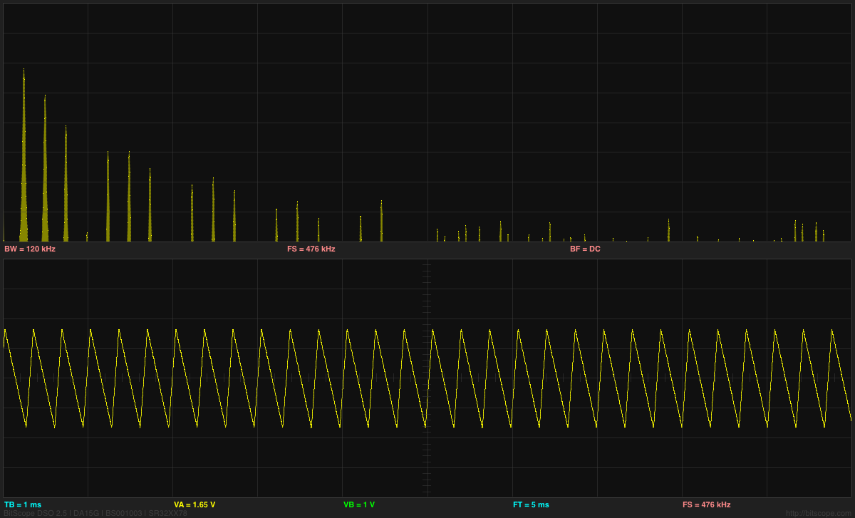
4. Sampling and Aliasing

   Students will use a PC board that samples and digitizes an input with an 8-bit ADC, then reconstructs the waveform with a DAC. An existing lab has been used in other EE courses for explaining and demonstrating aliasing of sampled signals using this board, a signal generator, and a dual-trace oscilloscope. Note: this is a student-executed demo, rather than a design or measurement lab.EE concepts: quantized time, quantized voltage, sampling frequency, Nyquist frequency, aliasing.

   Lab skills: dual traces on oscilloscope.Equipment needed: ADC/DAC board, dual-trace oscilloscope, function generator.

5. Audio amplifier

   Students will use an op amp to build a simple non-inverting audio amplifier for an electret microphone, setting the gain to around 6 or 7. Note that we are using single-power-supply op amps, so they will have to design a bias voltage supply as well.If this lab is too short, then students could feed the output of the amplifier into an analog input of the Arduino and record the waveform at the highest sampling rate they can with the software we provide (probably around 300–500 Hz). This would again demonstrate aliasing.EE concepts: op amp, DC bias, bias source with unity-gain amplifier, AC coupling, gain computation.

   Lab skills: complicated breadboarding (enough wires to have problems with messy wiring). If we add the Arduino recording, we could get into interesting problems with buffer overrun if their sampling rate is higher than the Arduino’s USB link can handle.

   Equipment needed: breadboard, op amp chip, assorted resistors and capacitors, electret microphone, Arduino board, optional loudspeaker.

6. Capacitive touch sensor

   The students will build an op-amp oscillator (a square-wave one, not a sine wave) whose frequency is dependent on the parasitic capacitance of a touch plate, which the students can make from Al foil and plastic food wrap. Students will have to measure the frequency of the oscillator with and without the plate being touched.

   Instead of breadboarding, students will wire this circuit by soldering wires and components on a PC board designed for prototyping op amp and instrumentation amp circuits.
   We will also provide a simple Arduino program that is sensitive to changes in the period of the oscillator and turns an LED on or off, to turn the frequency change into an on/off switch.EE concepts: frequency-dependent feedback, oscillator, RC time constants, parallel capacitors.

   Lab skills: soldering. Frequency measurement with multimeter.

   Equipment needed: Power supply, multimeter, Arduino, clip leads, amplifier prototyping board, oscilloscope.

7. Phototransistor

   The details of this lab have not been worked out yet. It will probably involve either making a photointerrupter switch or making and characterizing an optoisolater made from an infrared LED and a phototransistor.EE concepts: LEDs and phototransistors (maybe also photodiodes and photoresistors), optoisolators.

   Equipment needed: breadboard, LED, phototransistor, resistors, function generator, oscilloscope, multimeter.

8. Pressure sensor 1—instrumentation amplifier

   Students will design an instrumentation amplifier with a gain of 300 or 500 to amplify the differential strain-gauge signal from a medical-grade pressure sensor (the Freescale MPX2300DT1), to make a signal large enough to be read with the Arduino A/D converter. The circuit will be soldered on the instrumentation amp/op amp protoboard.The sensor calibration will be checked with water depth in a small reservoir. Note: the pressure sensor comes in a package that exposes the wire bonds and is too delicate for student assembly by novice solderers. We will make a sensor module that protects the sensor and mounts the sensor side to a 3/4″ PVC male-threaded plug, so that it can be easily incorporated into a reservoir, and mounts the electronic side on a PC board with screw terminals for connecting to student circuits.

   EE concepts: differential signals, twisted-pair wiring, strain gauge bridges, instrumentation amplifier, DC coupling, gain.

   Equipment needed: Power supply, amplifier prototyping board, oscilloscope, pressure sensor mounted in PVC plug with breakout board for easy connection, water reservoir made of PVC pipe, secondary containment tub to avoid water spills in electronics lab.

9. Pressure sensor 2—modeling fluidics with linear circuits
   Students will use the pressure sensors and amplifiers from the previous labs to characterize a pair of water reservoirs connected by a flexible hose. The details of the lab are still being worked out.Students will either induce a step change in pressure in one reservoir and record the step response in each reservoir, or will mount one reservoir on a homemade shaker table driven by a function generator and an audio amplifier.EE concepts: hydraulic analogy, frequency response (both amplitude and phase).

   Equipment needed: Power supply, amplifier prototyping board, oscilloscope, Arduino, pressure sensor mounted in PVC plug with breakout board for easy connection, 2 water reservoirs made of PVC pipe, hose connections, secondary containment tub to avoid water spills in electronics lab, possibly home-made shaker table. Note: the shaker table and power amplifier is the most expensive piece of equipment not already in the lab: it will cost about $50 to build.

10. Electrocardiogram EKG

    Students will design and solder an instrumentation amplifier with a gain of 2000 and bandpass of about 0.1Hz to 100Hz. The amplifier will be used with 3 disposable EKG electrodes to display EKG signals on the oscilloscope and record them on the Arduino.Equipment needed: Instrumentation amplifier protoboard, EKG electrodes, alligator clips, Arduino, oscilloscope.

3. Systemwide Senate Regulation 760 specifies that 1 academic credit corresponds to 3 hours of work per week for the student in a 10-week quarter. Please briefly explain how the course will lead to sufficient work with reference to e.g., lectures, sections, amount of homework, field trips, etc. [Please note that if significant changes are proposed to the format of the course after its initial approval, you will need to submit new course approval paperwork to answer this question in light of the new course format.]

This is a 2-unit course. Three hours a week will be spent in scheduled labs, another 3 hours a week in pre-lab design activity and post-lab write-ups.

4. Include a complete reading list or its equivalent in other media.

Wikipedia book: http://en.wikipedia.org/wiki/User:Kevin_k/Books/applied_circuits
Because no existing textbook covers all the material of the course, collection of relevant Wikipedia articles has been made that covers all the major topics. The book is available online for free, but students can purchase a printed and bound version (about 350 pages), if they want. Some of the Wikipedia articles contain more detail than is needed for the course, but about 90% of the content is relevant and will be required.

Data sheets: Students will be required to find and read data sheets for each of the components that they use in the lab.

Op amps for everyone by Ron Mancini http://www.e-booksdirectory.com/details.php?ebook=1469 Chapters 1–6 This free book duplicates some of the material in the Wikipedia book, but provides more detail and a cleaner presentation of some of the op-amp material.

Op Amp Applications Handbook by Analog Devices http://www.analog.com/library/analogDialogue/archives/39-05/op_amp_applications_handbook.html has some useful material, particularly in Sections 1-1 and 1-4, but is generally too advanced for a first circuits course. Readings in this book will be optional for the more advanced students.

The classic book The Art of Electronics by Horowitz and Hill has one of the best presentations of op amps in Chapter 4. Chapters 1 and 4, and parts of Chapters 5 and 7 are relevant to this course. Unfortunately, the book is now 23 years old and much of the description of specific chips is obsolete, but the book is still quite expensive. We will provide page and section numbers for optional readings in this book that correspond to the readings in the main texts, but not require this book.

5. State the basis on which evaluation of individual students’ achievements in this course will be made by the instructor (e.g., class participation, examinations, papers, projects).

Students will be evaluated on in-lab demonstrations of skills and on the lab write-ups.

6. List other UCSC courses covering similar material, if known.

EE 101L covers some of the same basic electronic lab skills, but without the focus on sensors or design, and without instrumentation amps.

Physics 160 offers a similar level of practical electronics, but focuses on physics applications, rather than on bioengineering applications, and is only offered in alternate years.

7. List expected resource requirements including course support and specialized facilities or equipment for divisional review. (This information must also be reported to the scheduling office each quarter the course is offered.)

The course will need the equipment of a standard analog electronics teaching lab: power supply, multimeter, function generator,  oscilloscope, and computer plus soldering irons. The equipment in Baskin Engineering 150 (used for EE 101L) is ideally suited for this lab. There are 24 stations in the lab, but only 12 function generators. Adding a dozen $300 function generators would make all 24 stations simultaneously usable, but the lab could be run with only half the stations, if all labs requiring function generators are done only with student pairs rather than individuals.

In addition, a few special-purpose setups will be needed for some of the labs. The special-purpose equipment was designed to be easily constructed with simple tools and to cost around $50/setup. One of the teachers is prototyping all the lab setups at home, to make sure that they can be effectively made within budget without expensive parts or much shop time.

There are a number of consumable parts used for the labs (integrated circuits, resistors, capacitors, PC boards, wire, and so forth), but these are easily covered by standard School of Engineering lab fees.

The course requires a faculty member (simultaneously teaching the co-requisite Applied Circuits course) and a teaching assistant (for providing help in the labs and for evaluating student lab demonstrations).

8. If applicable, justify any pre-requisites or enrollment restrictions proposed for this course. For pre-requisites sponsored by other departments/programs, please provide evidence of consultation.

Students will be required to have single-variable calculus and a physics electricity and magnetism course. Both are standard prerequisites for any circuits course. Although DC circuits can be analyzed without calculus, differentiation and integration are fundamental to AC analysis. Students should have already been introduced to the ideas of capacitors and inductors.

9. Proposals for new or revised Disciplinary Communication courses will be considered within the context of the approved DC plan for the relevant major(s). If applicable, please complete and submit the new proposal form (http://reg.ucsc.edu/forms/DC_statement_form.doc or http://reg.ucsc.edu/forms/DC_statement_form.pdf) or the revisions to approved plans form (http://reg.ucsc.edu/forms/DC_approval_revision.doc or http://reg.ucsc.edu/forms/DC_approval_revision.pdf).

This course is not expected to contribute to any major’s disciplinary communication requirement.

10. If you are requesting a GE designation for the proposed course, please justify your request making reference to the attached guidelines.

No General Education code is proposed for this course, as all relevant codes will have already been satisfied by the prerequisites.

11. If this is a new course and you requesting a new GE, do you think an old GE designation(s) is also appropriate? (CEP would like to maintain as many old GE offerings as is possible for the time being.)

No General Education code is proposed for this course, as all relevant codes (old or new) will have already been satisfied by the prerequisites.