Every machine has its own way of communicating with its operator. Some send status emails, some illuminate, but most of them vibrate and make noise. If it hums happily, that’s usually a good sign, but if it complains loudly, maintenance is overdue. [Ariel Quezada] wants to make sense of machine vibrations and draw conclusions about their overall mechanical condition from them. With his project, a 3-axis Open Source FFT Spectrum Analyzer he is not only entering the Hackaday Prize 2016 but also the highly contested field of acoustic defect recognition.

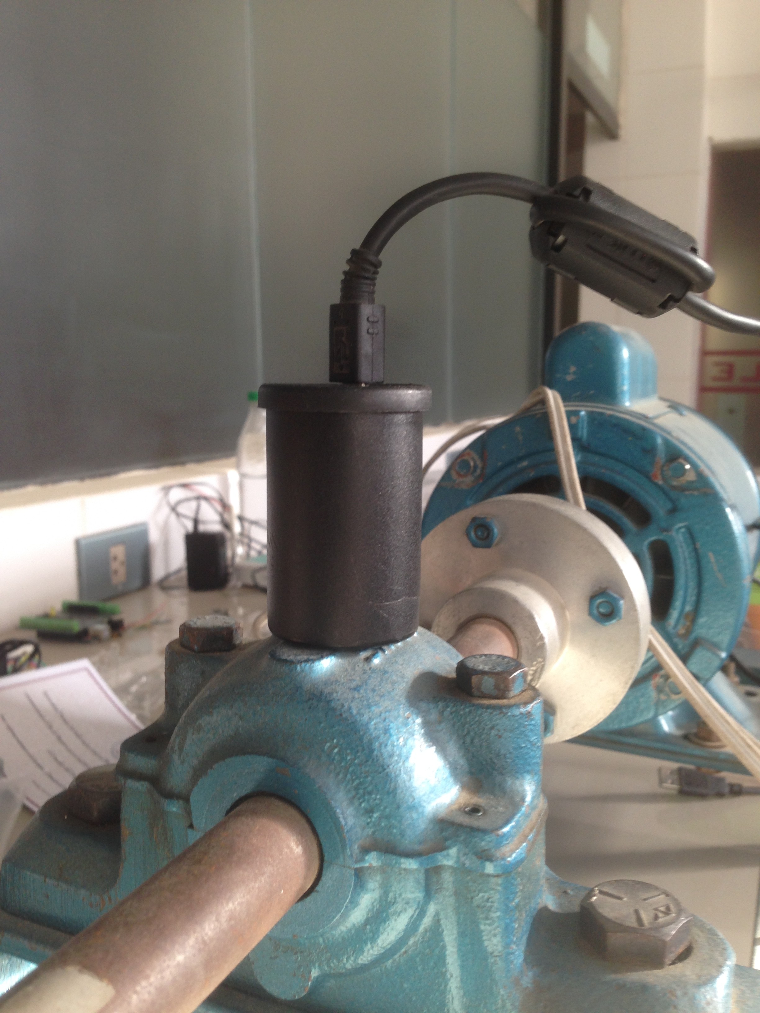
For the hardware side of the spectrum analyzer, [Ariel] equipped an Arduino Nano with an ADXL335 accelerometer, which is able to pick up vibrations within a frequency range of 0 to 1600 Hz on the X and Y axis. A film container, equipped with a strong magnet for easy installation, serves as an enclosure for the sensor. The firmware [Ariel] wrote is an efficient piece of code that samples the analog signals from the accelerometer in a free running loop at about 5000 Hz. It streams the digitized waveforms to a host computer over the serial port, where they are captured and stored by a Python script for further processing.

From there, another Python script filters the captured waveform, applies a window function, calculates the Fourier transform and plots the spectrum into a graph. With the analyzer up and running, [Ariel] went on testing the device on a large bearing of an arbitrary rotating machine he had access to. A series of tests that involved adding eccentric weights to the rotating shaft shows that the analyzer already makes it possible to discriminate between different grades of imbalance.

Yesterday, my son was thinking of adding a microphone to the design he is working on, and was considering adding a fast Fourier transform (FFT) to detect pitch.

He spent a few hours after his 10 a.m.–5 p.m. theater class reading about the FFT algorithm. He found an implementation of the FFT for an Arduino, which he tried reading along with the FFT explanations he found on the web.  I’m actually surprised the the Arduino was capable of doing an FFT, given the slowness of the processor.  It is true that the example code only does a 64-sample FFT with a sampling rate of 1kHz, using 8-bit samples and 16-bit integer arithmetic, but it is reported to do it at better than 10 FFTs per second.

I also pointed him to the Discrete Cosine Transform (DCT), which has somewhat smaller boundary artifacts, and can be computed about twice as fast, but he hasn’t had time to read that yet.  Somewhat surprisingly the DCT article in Wikipedia much better written than the general one on Fourier Transforms, which uses awkward notation and a rather dry, formal factoid dump.

I wanted to show him that FFT did not make pitch extraction trivial (at least not in real musical contexts), so I wired up a microphone and amplifier to my BitScope Pocket Analyzer and we turned on some Internet radio (our local public radio station, KUSP).  The complex mass of rapidly shifting peaks in the FFT made it clear that tracking a pitch would not be easy.  (I think that there are some useful pitch-extraction algorithms that are based on FFT, but they are not trivial.) I think I convinced him that he is better off trying to extract loudness than pitch, if he wants a useful control parameter for his device.

Incidentally, he spent some time yesterday looking for cheap electret microphones. There are quite a few on the market, but many of them say “hand solder only” on the datasheets—even some of the ones with just solder pads! There are mics that can be reflow soldered, but finding prices for them in the 100s is difficult—they mostly seem to be quotes from the manufacturers only. One promising one is the SiSonic SPQ2410HR5H-PD, which is only  3.76mm by 2.24mm and uses a ball grid array (it costs 92¢ in 100s, substantially more than 57¢ for the cheapest through-hole mic (though that needs to be hand soldered). CORRECTION 2013 July 10—that’s a MEMS silicon mic, not an electret.

We looked at digital mics that do the A-to-D conversion already, but the only one with a useful output format was the ADMP441, which costs $4.52 in 100s (way too expensive). The cheaper (down to about $1.02) digital mics all use PDM (pulse-density modulation), but to get that into a usable form inside the ATMega, he’d have to low-pass filter it and pass it through the A/D converter. Still, that may not be any more expensive than an analog mic, DC-blocking high-pass filter, and amplifier, though using a separate amplifier would let him design for the proper microphone sensitivity.  He’s going to have to figure out whether the board area and parts cost are worth the extra functionality of the microphone.  If the board area is not a problem, he could design the mic in, but then have the devices only partially populated to save parts costs, if necessary.

We also noticed that we could tell the bandwidth of the radio station we were listening to, because there was a very clear drop in the spectrum at 10kHz.  I tried capturing that this afternoon, but the station we listened to had a talk program rather than a music program, and I never captured a moment when they were using the full bandwidth.  I tried a different Internet music source, and got the following plot, which seemed to indicate a 12kHz bandwidth, but that may have been limited by the music recording they were playing, rather than the codec used for transmission over the internet.

Snapshot of FFT showing a bandwidth of about 12kHz. The grid for the spectrum is 10dB per division vertically and 6kHz per division horizontally.

Before we’d played with sound input, we’d looked at sine waves generated by the BitScope, by connecting a wire from the GEN output to the CHA input. I don’t think I was able to explain to him why the windowing function used for removing boundary artifacts in the FFT results in spreading the single-frequency spikes into wider peaks. It was too late at night to go into the theory of transforms and how multiplication in the time domain turns into convolution in the frequency domain, and vice versa. For that matter, he hasn’t even had convolution yet, so some of the fundamentals needed for the explanation were missing.

At one point I thought that the FFT on the Bitscope was a crude rectangular window, but I was informed by the Bitscope people that they use a Kaiser window. I should have been able to tell that they were doing some sort of windowing by seeing the spread of the spikes for sine waves, but I wouldn’t have been able to guess which window. (It may be buried in the documentation somewhere.) Actually, now that I look at the spikes, they seem too wide for a Kaiser window, unless they set the α parameter much too large.  They only need the sidelobes to be about 60dB down, which should be a much narrower main lobe—not the 18-bin width I think I’m seeing. Perhaps there is something else spreading the peaks, not just the Kaiser window.

Sine wave and FFT analysis of it (Click on image for larger, clearer picture). Note the harmonic distortion (2nd, 3rd, and 4th harmonic at about –40dB, –45dB, and —53dB).
Good luck figuring out the settings of the Bitscope from the information they show on the display!  TB is the time per division on the x-axis of the plot, while BW=120kHz is the full width of the spectrum (so 12kHz per division), and the sine wave is at about 3kHz.

It is interesting to look a a sine wave that is an exact submultiple of the sampling frequency:

Here is a 2975Hz sine wave, where each period should be 8 samples long. Note the appearance of side bands to either side of the main peak. These artifacts are much smaller if we move to a frequency that does not fit so neatly into the FFT buffer.
Note that the time base is different for this screenshot (20ms/division).

We also looked at the spectra of triangle waves and square waves (since the BitScope waveform generator can do those also). Playing with the duty cycle was fun also. I had not been aware that a duty cycle of 1/n on a square wave or triangle wave suppressed the nth, 2nth, 3nth, … harmonics. I had known that a 50% duty cycle square wave or triangle wave suppressed the even harmonics, but I had never thought about other duty cycles.

Triangle wave with 25% duty cycle, showing suppression of the 4th, 8th, 12th, and 16th harmonics.

Yesterday, my son was thinking of adding a microphone to the design he is working on, and was considering adding a fast Fourier transform (FFT) to detect pitch.

He spent a few hours after his 10 a.m.–5 p.m. theater class reading about the FFT algorithm. He found an implementation of the FFT for an Arduino, which he tried reading along with the FFT explanations he found on the web.  I’m actually surprised the the Arduino was capable of doing an FFT, given the slowness of the processor.  It is true that the example code only does a 64-sample FFT with a sampling rate of 1kHz, using 8-bit samples and 16-bit integer arithmetic, but it is reported to do it at better than 10 FFTs per second.

I also pointed him to the Discrete Cosine Transform (DCT), which has somewhat smaller boundary artifacts, and can be computed about twice as fast, but he hasn’t had time to read that yet.  Somewhat surprisingly the DCT article in Wikipedia much better written than the general one on Fourier Transforms, which uses awkward notation and a rather dry, formal factoid dump.

I wanted to show him that FFT did not make pitch extraction trivial (at least not in real musical contexts), so I wired up a microphone and amplifier to my BitScope Pocket Analyzer and we turned on some Internet radio (our local public radio station, KUSP).  The complex mass of rapidly shifting peaks in the FFT made it clear that tracking a pitch would not be easy.  (I think that there are some useful pitch-extraction algorithms that are based on FFT, but they are not trivial.) I think I convinced him that he is better off trying to extract loudness than pitch, if he wants a useful control parameter for his device.

Incidentally, he spent some time yesterday looking for cheap electret microphones. There are quite a few on the market, but many of them say “hand solder only” on the datasheets—even some of the ones with just solder pads! There are mics that can be reflow soldered, but finding prices for them in the 100s is difficult—they mostly seem to be quotes from the manufacturers only. One promising one is the SiSonic SPQ2410HR5H-PD, which is only  3.76mm by 2.24mm and uses a ball grid array (it costs 92¢ in 100s, substantially more than 57¢ for the cheapest through-hole mic (though that needs to be hand soldered). CORRECTION 2013 July 10—that’s a MEMS silicon mic, not an electret.

We looked at digital mics that do the A-to-D conversion already, but the only one with a useful output format was the ADMP441, which costs $4.52 in 100s (way too expensive). The cheaper (down to about $1.02) digital mics all use PDM (pulse-density modulation), but to get that into a usable form inside the ATMega, he’d have to low-pass filter it and pass it through the A/D converter. Still, that may not be any more expensive than an analog mic, DC-blocking high-pass filter, and amplifier, though using a separate amplifier would let him design for the proper microphone sensitivity.  He’s going to have to figure out whether the board area and parts cost are worth the extra functionality of the microphone.  If the board area is not a problem, he could design the mic in, but then have the devices only partially populated to save parts costs, if necessary.

We also noticed that we could tell the bandwidth of the radio station we were listening to, because there was a very clear drop in the spectrum at 10kHz.  I tried capturing that this afternoon, but the station we listened to had a talk program rather than a music program, and I never captured a moment when they were using the full bandwidth.  I tried a different Internet music source, and got the following plot, which seemed to indicate a 12kHz bandwidth, but that may have been limited by the music recording they were playing, rather than the codec used for transmission over the internet.

Snapshot of FFT showing a bandwidth of about 12kHz. The grid for the spectrum is 10dB per division vertically and 6kHz per division horizontally.

Before we’d played with sound input, we’d looked at sine waves generated by the BitScope, by connecting a wire from the GEN output to the CHA input. I don’t think I was able to explain to him why the windowing function used for removing boundary artifacts in the FFT results in spreading the single-frequency spikes into wider peaks. It was too late at night to go into the theory of transforms and how multiplication in the time domain turns into convolution in the frequency domain, and vice versa. For that matter, he hasn’t even had convolution yet, so some of the fundamentals needed for the explanation were missing.

At one point I thought that the FFT on the Bitscope was a crude rectangular window, but I was informed by the Bitscope people that they use a Kaiser window. I should have been able to tell that they were doing some sort of windowing by seeing the spread of the spikes for sine waves, but I wouldn’t have been able to guess which window. (It may be buried in the documentation somewhere.) Actually, now that I look at the spikes, they seem too wide for a Kaiser window, unless they set the α parameter much too large.  They only need the sidelobes to be about 60dB down, which should be a much narrower main lobe—not the 18-bin width I think I’m seeing. Perhaps there is something else spreading the peaks, not just the Kaiser window.

Sine wave and FFT analysis of it (Click on image for larger, clearer picture). Note the harmonic distortion (2nd, 3rd, and 4th harmonic at about –40dB, –45dB, and —53dB).
Good luck figuring out the settings of the Bitscope from the information they show on the display!  TB is the time per division on the x-axis of the plot, while BW=120kHz is the full width of the spectrum (so 12kHz per division), and the sine wave is at about 3kHz.

It is interesting to look a a sine wave that is an exact submultiple of the sampling frequency:

Here is a 2975Hz sine wave, where each period should be 8 samples long. Note the appearance of side bands to either side of the main peak. These artifacts are much smaller if we move to a frequency that does not fit so neatly into the FFT buffer.
Note that the time base is different for this screenshot (20ms/division).

We also looked at the spectra of triangle waves and square waves (since the BitScope waveform generator can do those also). Playing with the duty cycle was fun also. I had not been aware that a duty cycle of 1/n on a square wave or triangle wave suppressed the nth, 2nth, 3nth, … harmonics. I had known that a 50% duty cycle square wave or triangle wave suppressed the even harmonics, but I had never thought about other duty cycles.

Triangle wave with 25% duty cycle, showing suppression of the 4th, 8th, 12th, and 16th harmonics.

• Three 16-channel, 12-bit pwm PCA9685 chips will operate MOSFET's to switch 48 LED strips.
• Small sot23 smd MOSFETs (or these); the old ones (P16NF06's) were too overkill, too big. Overkill is still good but there's some math this time.
• RC batteries for more power: peak 14.8V and 12A no problem, but will be <500mA most of the time.
• Thinner, lighter LED strips with 120 LED's/m.
• Arm-based remote control with a 1.3" OLED screen, dials/buttons/sliders/TBD.
• The remote control will hopefully be a second Arduino-based system, a serial peripheral to the main suit system.
• Multi-band audio analysis with MSGEQ7 or a separate Arduino FFT.

It’s about right time to release one more “remix” for one of my blog, published almost a year ago. I haven’t got much comments, not many as I was expecting, on a topic. There are some reasons, that would explain this phenomenon, but I would better to start outlining what I did in new release, and some of you who tried old version would be impressed by progress I’ve made!

Basic structure was left almost intact. Essential parts of the project: Filtering 2D and Cross-Correlation are the same, so please read my old post, if you come across this one w/o seen it first. What differs is “preprocessing”, before we get to the filtering stage. In first, I ported a code on Leonardo board.  The easiness of connecting electret mic to Leonardo, just didn’t give me a choice!  I played already with Leonardo ADC – electret mic’s in my previous post, and would assure you, that this guys were designed to work as a team. Uno followers have to solder a pre-amplifier, not big deal, the same time not really interesting.  Code would run on Uno, except Timer and ADC settings, which you could always “copy/paste” from the old version. Feel free, be my guest.

Analog front-end is absolutely the same as I used in Sound Localization project. You would need only one mic here, just reduce the number of electrical components down.

Sampling subroutine based on Timer 4, and arduino Leonardo internal PGA set to gain x40. There are a comments in the code, so you could adjust gain up or down depends on the sensitivity of mic you have.

Windowing LUT is slightly modified Hamming/Hann cosine function,  I’d say my table is an “intermediate” version of both mention inventors.

FFT is my best achievements of this year, RADIX-4.  Compare to old code, about 3x faster. This is why I was able to increase FFT_SIZE up to 128,  still having plenty of time.  Magnitude calculation is based on approximation, very fast, because no square root extraction required. Accuracy, in the worst case scenario ~95%, which is more than enough in this project.

I changed Non-Linear compression algorithm, as now there are more Bins – 64 to pack in 16 Bands. Math is simple, and hope doesn’t need an extensive comments. Packing is necessary due memory limits, 1 sec password in current configuration (16 bands with sampling rate 4 kHz) occupied 1 kByte, full size of EEPROM on Leonardo or Uno boards.

Command Line Interface is preserved. Here is the instructions, how to set everything up and running.

And here how spectrogram looks like in LibreOffice, test phrase “Front right”, (OS Linux Ubuntu, 12.04):

Instructions.

 Get your microphone wired / connected? All checked at least a couple times with multimeter, voltages looks o’k? Good, now you are ready to start! ( Don’t forget to upload a sketch to your arduino / Leonardo -);

1. X. First of all, open serial monitor window, and check boadrate.
Should be 115200. Next, type “x” and Enter. Get some response? Does
it look like a table? Excellent, data you are looking at is “raw” 
sampling data. Probably, just noise, acoustical or electrical. 

2. F. Second test, type “f” - Enter. Again, arduino would print out 
a table. This time data represent “processed” by FFT analog signal. 
Each bin corresponds to frequency range 32 Hz. If you have a signal
generator , it's right time to do a detailed check up microphone, 
wiring, and software. If don't have, you can use your computer's 
sound card and some program, there are plenty of them available 
on-line free of charge. Connect generator to PC USB speackers, and
run a single tone, anything in audible range 16 – 2000 Hz. Check 
again using “f” command, if arduino registers a signal, and it's in
right bin. Due “windowing” function, even pure single tone would 
show up at least in 2-3 neighboring bins. Amplitude depends on 
sensitivity of the mic, and volume of the sound. Sending “x” you can 
confirm, that there is no “clipping” too many “– 511” or “+511”.

3. S. Next, if all goes well till this step, you probably already
notice, that whenever a mic picking-up a sound – yellow on-board LED
lights up. Now, it's better shutdown your TV, iPad, radio. 
Make your environment as quite as possible. Try to say something 
with your own voice, and see if led lighting up when you start 
talking, and than after ~1 sec it goes off. Repeat a few times, 
adjusting a volume and / or distance to the mic, so led goes “on/off”
reliable. Send “s” command when led is off. Don't worry, it should 
be no report on screen, till you say a word. Procedure is simple, 
send “s” - say something. After you talk, and get a printing, look 
carefully. Your objective, is get a “spectrogram” which consist of 
a few spots / blobs of digits, randomly distributed all over the 
“surface”. Repeat a few times with one word, than try another one 
and so on. With short words, very likely reporting data would be 
concentrated at the top ( you may need to scroll up to see the 
beginning), if this is a case, better to choose longer words or talk
in slower tempo. Just remember, there are three dimension, time, 
frequency and volume. You can use a signal generator here again, 
spectrogram should looks like a vertical line, may be 2 - 3 parallel
lines on low frequencies test tones. 
 Changing a frequency, you can even get some curves. What is 
important, the must be no negative numbers. If you see them – 
"overloading" happens, Decrease a volume. Dynamic range is limited 
by 127, more close you can get to this value w/o negatives, 
the better. And last dimension is a frequency. For man, it would 
be a little bit hard to “detach” a spectrogram from the left border.
It's true for everyone, who is not opera singer, me no exceptions.... 

4. R and G. After you practice enough, and received Manny nice 
looking spectrograms, it's time to check with arduino, if it's 
agree with you / thinks similar. Send “r” - recording, and say 
a word you've get your best spectrum with. Wait a few seconds, 
writing to EEPROM takes time. Now send a “g” and say the same word.
In the same manner, tonality and volume. See on the outputs, what 
is the cross-correlation factor you received. More than 50% - very 
good for beginning. Less – try again a few more times sending “g” and
repeating same word, maybe slightly varying pronunciation. Try to 
reach best recognition, “crack” your own password code! 
( note: Negatives number on “G” reports-form must be present.)
If no luck try another password code. Now you know the drill: 
S – repeat, repeat, repeat....., R, G – repeat, repeat, repeat..... 
(joke). Can't get good match? Try your computer's test sounds, 
beeps, horns, clicks, barks – whatever your OS has. It doesn't have
to be shorter than 1 sec, but only 1 second in the beginning 
would be stored / compared. My computer is able to repeat the same 
sound track (speakers test - "front right") with enormously high 
cross-factor 99 % ! I'm not a computer, my best short 86 % so far...

5. P. This command is simply reading the content of the EEPROM, 
so you always can verify, what you stored last time. 
Editing / formatting this data you can store a table in the arduino 
FLASH memory using PROGMEM. About 10 – 15 commands. Of course, 
storing data in external SD card or EEPROM, could greatly increase
the “vocabulary”, the same time design of fast cross-correlation 
algorithm with multiple “pattern”s would be another brain teasing
puzzle -);.

Have fun!

Link to arduino sketch, VOR (VOice Recognition).

Well, it’s elementary simple in theory, how to do sound localization based on phase difference of signals, that received by two spatially distant microphones. The devil, as always, in details. I’ve not seen any such project created for arduino, and get curious if it’s possible at all. Long story short, here I’d like to present my project, which answer this question  - YES!

Moreover, quantity  of electronics components not much differs from what I’ve used in my previous blog.  Compare two drawings, you will notice only 4 resistors and 4 electret microphones were added! All circuitry is just a few capacitors, 9 resistors, one IC and mics.  Frankly speaking, writing a remix of oscilloscope, I was testing  an arduino analog inputs, keeping in mind to use it in junction with electret microphones in other projects, like sound pressure measurements (dBA),  voice recognition or something funny in “color music” series. As they call it – “a pilot” project?.  There are some issue (simplest ever) oscilloscope has when doing fast rate sampling on 4 channels (settings 7, 8 and 9 Time/Div ) I already described, so I slightly reduce sampling down to 40 kHz here.

Note: *Hardware would be different for arduino boards based on different chips, and must include pre-amplifiers with AtMega328 uCPU. 

One more important things to mention in this short introductory, as I used FFT algorithm for phase calculation ( I like FFT very much, you probably, already notice it ),

Arduino is capable not only track a MOSQUITO flying in your room, it could tell if it’s MALE of FEMALE !!!!!

                  SOFTWARE.

  As I say above, I choose 40 kHz for sampling rate, which is a good compromise between accuracy of the readings  and maximum audio frequency, that Localizator could hear. Getting signals from two mic’s simultaneously, upper limits for audio data is 10 kHz. No real-time, “conveyor belt” include 4 major separate stages:

• sampling X dimension;
• FFT
• phase calculation
• delay time extracting

• sampling Y dimension;
• FFT
• phase calculation
• delay time extracting

4 mic’s split in 2 groups for X and Y coordinate consequently. Picking up 4 mic’s simultaneously is possible, but would reduce audio range down to 5 kHz, so I decided to process two dimension (horizontal and vertical planes)  separately, in series. Removing vertical tracking from the code, if it’s not necessary, would increase speed and accuracy in leftover plane, of course. I’d refer you for description of the first and second stages to other blogs, FFT was brought w/o any modification at all. Essential and most important part of this project, stages 3 and 4.

Phase Calculation (3).

 Mathematical tutorial on a topic, I’m not any good as a teacher, so you better read somewhere else, to brush up a basic concept. Core of the process is arctangent function. This link says a number of cycles. In two words – too slow.  LUT ( Look Up Tables ) is the best solution for no-float uCPU to do complex math extremely fast, and reasonably (?) precise. Drawback of LUT is limited size, so it could be saved in FLASH memory, which in next tern  is also limited. This is what I did on “resource management” side: 1 kWords ( 16-bit integers, 2 kBytes) , 32 x 32 ( 5 x 5 bites) LUT, scaled up to 512 to get better “integer” resolution. There are a few values in top-right corner, that melted together as their differences are less than “1″ (not shown on the picture on right side). The “worst” resolution is in top-left corner, where “granularity” is reaching 256, or unacceptable 50% of the dynamic range. To stay as far away from this corner, I put a “Rainbow Noise Canceler” – single line with ” IF ” statement, which “disqualifies” any BIN with magnitude, calculated at the FFT stage, lower than 256.

IF(((sina * sina) + (cosina * cosina)) < 256) phase = -1;

 I called it “Rainbow” because of it’s shape, “red line” is an arc, going from 16 on top line to 16 on left side. Also, “Gain Reset” – 6 bit ( depends on the FFT size, has to be 6 bits for 128) reduced to 5 bits, in order to get better sensitivity. This two parameters / settings, 5-bit and 3.5 bit magnitude limit, create a “threshold” for weak spectral peaks. Basically, depends on application, both values can be adjusted in  different proportions.

 There are two category of tracking technics, with mic’s installed on moving platform, and stationary mic’s. First one is a little bit easier  to understand and build, requires Relative direction to sound source. This what I’ve done. Stationary mic’s approach, when motors are moving laser pointer (or filming camera) alone, would require Absolute direction to sound source, and must include stage #5 – angle calculation via known delay time. Math is pretty simple, acrsine function, and at this point only one calculation per several frames would be necessary, so floating point math wouldn’t be an issue at all. No LUT, scaling, rounding/truncation. Elementary school geometry knowledge – thats all you need.

Delay Time Extraction (4).

 Subtraction phase value of one “qualified” mic’s data pull from another, produce phase difference. To turn phase difference in delay time, division by BIN number is performed. Lets call this operation “Denominator” process.  The denomination is necessary, because all data after this step going to be combine and process together, doesn’t matter of wave length, which is different for every bin. Frequency and wavelength related to each other via simple formula:  Wavelength = Velocity / Frequency, where velocity is a speed of sound wave in the air ( 340 m/sec at room temperature). As distance between two mic’s is a constant,  sound with different wavelength ( frequency ) produce different phase offset, and denomination make them proportional. (WikiPedia, I’m sure, would explain this much better, mind you, I’m a Magician, not mathematician).

First picter on right side shows  ”Nuisance 3: Incorrect arctan” correction. You will find two lines with “IF” statements in the code relaited to stage #3.

Second one,  gives you idea why other correction at stage #4 is necessary As you can see, subtraction one arctan from another generates a rectangular “pulse” ( Diff. n. corr., violet line) whenever one function changes sign but other (delayed version) not yet. Light blue line (DIFF(B)) doesn’t have such abnormality. Math is simple, just two lines with “IF’s” in the same manner, only “double size” constants this time. 2048 on my scale corresponds to 2 x PI, 1024 – PI, and 512 – PI / 2.

Arduino has only 1 ADC, so there is always constant delay time equals to one sampling period ( T = 1/40 kHz = 25 usec), which also should be subtracted ( or added, depends how you associate input 1 and 2 – left / right side mic.)

Filtering.

 To fight reverberation and noise, I choose a Low Pass Filter, which I’d call here as a “Rolling Filter”. My research with regular LPF, shows that this class of filters is completely NOT appropriate for such type of data, due their high susceptibility to “spikes”, or sudden jump in magnitude level. For example, when system getting steady reading from 2-3 test frequencies with low values, let say -10, simple averaging ( should be -10 ) results will be corrupted with one accidental spike (magnitude +2000) during next 60 – 100 consecutive frames !!!  The Median Filter doing well eliminating sudden spikes, the same time is very hungry to CPU cycles, as it’s using “sort” algorithm each time new sample was arrived to the data pull. Having 64 frequencies, and setting filter kernel to 5 – 8 samples, arduino would be buried doing sorting at almost 40 ksps.  Even processing each frequencies data not individually,  and sorting only one 64 elements array still very time consuming job.  After thinking a while, I came up to conclusion, that “Rolling Filter” has almost the same efficiency as Median, but instead of “sorting” requires only 1 additive operation! On long run, the output value will “roll” and “stick” to the middle of the pull. ( Try to model it in LibreOffice. )  Adjusting “step” of the “Rolling Filter”, you can easy manipulate responsiveness,  which is almost impossible with Median Filters. (Things TO DO: Adaptive Filtering, real time adjustment depends on input data “quality”).

 To be continue…. Video will follows !

( Predicting your question, how “good” is localization?  Its about same, as Laser TRF (tracking range finder) has, look at other blogs for now to get impression.  In other words: ASTONISHINGLY GOOD,   a few (1 – 5) angular degree in closed environment.

Link to Arduino (Leonardo) sketch:  Localizator-beta-9.

O’K, after having some fun with stereo version of the VU meter I described in my previous blog-post, now it’s time to do a serious stuff. Studio grade VU meter !!! 24 steps, equally spaced every 3 dB, covering Extra wide Dynamic Range from -63  up to  +6 dB.  Single (mono) channel this time, no messing around, absolute precision at the stake. Plus, it keeps absolutely Top-Flat linear frequency response from 40 Hz up to 20 kHz(*).

I’m not going into details of RGB LEDs Display, which has no modification since “Tears of Rainbow” project, only plates installed in one line, form a single GIGANTIC bar-graph. There are some minor changes in mixing colors data tables, but they intuitively understandable.  The most important feature in this project is autoscaling. As you, probably know, Arduino has 10 bits ADC. Only it can’t process negative half-wave, and for this reason it has only 9 bits available for AC measurements.  According to DSP theory, maximum dynamic range is:

DR = 1.77 + 6.02 x B = 1.77 + 6.02 x 9 = 55.95 dB.

 As input audio waveform represents anything but perfect peak-to-peak 5V sine-wave, real dynamic range would be lower. How much? In first, there is a hardware limits.  OPA (NE5532), which is:

• very low noise !!!
•  high output-drive capability;
•  high unity-gain and maximum-output-swing bandwidths;
•  low distortion;
•  high slew rate;
•  input-protection diodes, and output short-circuit protection

 but, unfortunately,  isn’t rail-to-rail type. Test results show, that compression  become noticeable (~1 dB) when not scaled magnitude approaches level about 50 dB. That is in good agreement with observed on oscilloscope not distorted deviation peak-to-peak 2.5 V. Or only half of full range of 5V. And as theory says, half is one bit less, and real DR = 1.77 + 6.02 x 8 = 49.93  (~50 dB). In second, audio data is processed on “block” structure basis. It means, having average of the block 50 dB, doesn’t mean that there was no spikes in the sampling pull, that obviously would be clipped and introduce error in the measurements results.  This phenomenon is defined as Crest Factor. Different sources estimate crest factor of musical content between 10 – 20 dB.  So, taking direct approach, Arduino with OPA mentioned above as front-end could accurately cover only:              50 – 20 = 30 dB.  To get wider dynamic range, I have to scale input amplifier gain, and this is exactly what I did, building amplifier in two stages and selecting one cascade (by-passing second one) or two cascades using internal ADC multiplexer. As there is no switching IC in analog signal path involved, gain is defined with high stability, could be one time precisely measured – calibrated via coefficient stored in EEPROM (nice feature to add).

On the right side there are electrical drawings of “slightly” modified kit,  where stereo amplifier was converted into 2 stage mono version. First stage, with gain about  G1 = 1 + 10 k / 1 k = 11  is necessary to “bump-up” line-level signal, to create DC bias required for correct operation of the ADC, and also served as buffer to lower signal source impedance, as it seen by ADC input.  I set a gain of the second stage amplifier at 40 dB:  20 x Log_10 ( G2 ),     where    G2 = 1 + 100 k / 1 k = 101.

IMHO, setting gain limit for only 30 db per stage as it follows from paragraph above, is overkill, and would be justified for “real-time” radio broadcasting or audio processing for storage media, when high fidelity of audio program must be preserved. For visual display “clipping” of bursts in signal is not noticeable at all due high refresh rate of display, 78 Hz. Human just can’t see, if LED lights-up with such speed.  For steady AC amplitude measurements (micro Voltmeter mode) this is not a problem at all, and headroom as small as 3 dB would be sufficient, leaving wide 47 dB per stage.

 Software

  There are two thresholds are defined in program, where switching between one or two stage amplification is happening:

      if ( magn_new <=  44 ) sensitv = 1;

      if ( magn_new >= 47 ) sensitv = 0;

  44 and 47, with hysteresis 3 dB. First line defines switching to high sensitive mode (overall gain 1100), and second line, does exactly opposite. Look at the chart, hope it would save me a million words -);

 Couple words on using this device as precise AC micro-voltmeter. Having 1100 overall amplification as add-up to already quite sensitive Arduino ADC, driving overall sensitivity to enormously  5 / ( 1024 x 1100 ) = 4.439 uV Special care should be taken on grounding, shielding of amplifier PCB, probably, EMI suppressor ferrite chokes wouldn’t be an excess in power line and signal path.   In my project, w/o any modification to original kit’s board (except couple jumper wires to cascade two stage amplifier) of course, I was not expecting to get to such high sensitivity level. Moreover, in project arduino is driving LED display, “ADC noise reduction mode” is off, plus ADC is working on double speed – preselector set to 250 kHz!!!  And this is why constant 14 was subtracted in software from magn_new, just before it goes for BarGraph “mapping” procedure:

      magn_new  -= 14;

Basically 14 is a noise flour of my analog front-end.  Approximately 51 micro volts AC is turning on first LED bar. Look at the table, which reflect my current hardware set-up.

* Other things to keep in mind, there is a “gap” 78 Hz wide in frequency range at 10 kHz,  It introduces a small error, about  78 / 20.000 = 0.39% in white noise measurements result. For musical content, which has really low power density level at 10 kHz, magnitude of error would be much lower, probably, less than 0.05 %.

 Running FFT in code creates great opportunity to reject any interference in the audio band. For example, if there is a noticeable hum from electrical grid lines in the content, issue easily could be fixed NOT including bin[1] in final sum of magnitude calculation. Though to make it works more efficient, some adjustment in sampling period would be necessary, setting bin[1] frequency precisely at 50/60 Hz.

 One more advantage of having FFT based  filtering     (primary mission is HPF, look in stereo VU meter, how long kernel of the FIR filter has to be otherwise), is great opportunity to create “weighting” A, B, C or D curve for audio noise measurements. (:TO DO).

 Link to Download Arduino sketch:  Audio_VU_Meter_Mono_69dB

This blog is a sequel of “Tears of Rainbow”.  Using the same hardware set-up of Gigantic RGB LED display, I decided to re-work software a little bit, in order to display the true RMS amplitude of musical content. Video clip on youtube:                       VU_Meter   640×480                                      VU_Meter_HD

Objective:

• Stereo input, process both channel;
• Full audio band, 40 Hz – 20 kHz;
• Fast update rate of visual output.
• Precision Full-Wave  measurements. 

To process stereo input, this time arduino is switching ADC multiplexer every time when it finish sampling input data array (size=128). Two channels “interleaved” with frame rate 78 Hz, so during each frame only one channel sampled / processed, and update rate per channel is equals to 78 / 2 = 39 Hz, which is more than enough for most audio applications.

 I’m using FFT Radix-4  to extract RMS magnitude of audio waveform, and this is why:

1.  Sampling rate in this application is 10 kHz. How I achieved  20 kHz stated in objective section, doing sampling only 10 ksps?  >>>Aliasing!<<<   What is considered to be nightmare when we need spectral information from FFT output, aliasing in this project is really helpful, reflecting all spectral components around  axis – 10 kHz back “to the field”. As all bins going to be sum-up there is no issue, only benefits. Due aliasing, I’m able to use low sampling rate, and reduce CPU workload down to 52%.

2.  In order to get accurate magnitude calculation of RMS,  which is defined as square root of the sum of squares divided by number of samples per specified period of time:    V(rms) = √ ( ∑ Vi ^2 ) / N) DC offset  must be subtracted from the input raw data of each sample    Vi = Vac + Vdc   (if you remember, AtMega328 ADC needs DC offset to read AC negative half-wave).  The problem here, DC offset value is never known with high accuracy due bunch of reason, like voltage stability of PSU,  thermal effects, resistors tolerance (+/- 1 or 5 %), ADC internal non-linearity etc. Cure for this, which works quite well for monitoring electrical grid power, high pass filter (HPF). Only instead of single 50/60 Hz frequency of power line,  I have a wide frequency range, starting from 20 Hz and ending at 20 kHz. When I feed specification of the HPF:

• Sample Rate (Hz) ? [0 to 20000]                     ? 10000
• Desired stop-band attenuation (dB) [10 to 200] ? 40
• Stop-band edge frequency Fa [0 to 5000]         ? 0
• Pass-band edge frequency Fp [0 to 5000]        ? 40

to  Parks-McClellan FIR filter design algorithm (one of the most popular, and probably, the best) it provides the result:

• …filter length: 551 …beta: 3.395321

551 coefficient to be multiplied and sum up (MAC-ed) every 100 usec! No way. I’m not sure, if it could be done on 32-bits 100 MHz platform with build-in MAC hardware, but there is no way for 8-bit 16 MHz Arduino.

IIR filter wouldn’t make much difference here. It has lower quantity of multiplications, but more sensitive for truncation and rounding error, so I’d have to use longer (32-bits?) variables, which is not desirable on 8-bit microprocessor at all.

And here comes FFT Radix-4, which easily fulfill this extra-tough requirements in the most efficient and elegant way. All I have to do, is just NOT include bin[0] in final sum, and all DONE!. TOP-FLAT  linear frequency response  40 Hz – 20 kHz  ( -3 dB ), with complete suppression of DC, and low frequency rumble below 20 Hz attenuation.  Linearity is better than +-1 dB between 80 – 9960 Hz.

Last things, audio front-end. As VU meter was designed in stereo version, I’ve build another “line-in”  pre-amplifier based on this kit: Super Ear Amplifier Kit

Video clips on youtube, arduino is running simple demo application.

Tears of Rainbow                             BarGraph HD movie                                    " href="//www.youtube.com/watch?v=30ELYwyy4JQ&feature=youtu.be]" target="_blank">BarGraph movie.

It’s time to release new updates for my first (ever) project with Arduino, “Color Light Music”.  From artistic perspective, VU BarGraph style (IMHO) is the best one for spectral dynamic representation, and not much could be improved on this side. But this time, it cross my mind an another idea “Tears of Rainbow”. This blog about how successively (or awfully) the idea was brought to life. And of course, VU visual effects still there, updated with nice peak indicators, color adjustment flexibility (this time triple color LEDs), and PWM-ed brightness settings luxury.  So, this is design requirements, I was following:

•   make it as big as possible, GIGANTIC size !;
•   Lego style, or many blocks / modules, which could be re-arranged in different pattern;
•   extend-able,  easy to add up more blocks later on;
•   low price on hardware, no special display driver IC.

        * For clarity, schematic diagram shows only two pairs of chip, and half length of the strip lines.

Now software part.

There are on-line libraries available, to drive 74HC595 by arduino. Only some of them not using hardware “build-in”  SPI interface , and really slow in communication with peripheral IC’s (don’t forget, that LED display only second part of the project, the first one, FFT, is very time consuming). The others libraries, nicely written and perfectly optimized for speed, have too much functionality, that I don’t need in my project, plus they are memory demanding. On the other hand, I need low resolution animation function – sliding down colorful tears, that I have to create on my own.  Now I ‘d like to represent a code, very fast SPI subroutines, completely written in C !  Function shift out 9 bytes ( for 9 shift registers in this project ) approximately in less than 36 usec, or 0.5 usec per one PWM channel. One bit-set in the unrolled loop is about 4.5 cycles.

static uint8_t brightn;

brightn++;
 if(( brightn % QUANTUMS ) == 0)
{
bitClear(PORTB,LATCH_PB);
SPDR = 0;

uint8_t * srP = &brightns[PIN_NBRS];
uint8_t cmp_level = brightn;

for (int8_t iSR = 0, curBt = 0; iSR < IC_COUNT ; iSR++, curBt = 0){

if ((* –srP) > cmp_level)
curBt |= 0b00000001;
if ((* –srP) > cmp_level)
curBt |= 0b00000010;
if ((* –srP) > cmp_level)
curBt |= 0b00000100;
if ((* –srP) > cmp_level)
curBt |= 0b00001000;
if ((* –srP) > cmp_level)
curBt |= 0b00010000;
if ((* –srP) > cmp_level)
curBt |= 0b00100000;
if ((* –srP) > cmp_level)
curBt |= 0b01000000;
if ((* –srP) > cmp_level)
curBt |= 0b10000000;

loop_until_bit_is_set(SPSR, SPIF);
SPDR = curBt; // Start the transmission
}
loop_until_bit_is_set(SPSR, SPIF);
bitSet(PORTB,LATCH_PB);
}

FFT part of the code completely “copy / pasted” form my “Radix-4″ blog. Here an advise, if you wish to explore the code, look there for “pure” form of function. What is new in this publication, is magnitude calculation subroutine, without slow SQRT.

Bar Graphs “set position” sub-function, or mapping height of lighted area of a plate to integral sum of the bins, brought into this project with mild modification from first project.

Continue moving from LED’s display to audio input, I should say couple words on a sampling. There are two functions in the project, that have to be triggered periodically with a timer, “display refresh” posted above and “take ADC sample”. It looks logically, instead of having two timers and have a lot of troubles with collision / racing between them, to scale both function to the same time frame, and execute them at once. “Display refresh” rate equals to minimum rate just to avoid flickering (60/70 Hz) multiplied by the numbers of brightness level. For example, setting brightness step number to 256 ( which provides excellent 256 x 256 x 256 = 16 M colors ) would require periodicity 60 x 256 = 15360 Hz.  See, where I’m driving at? Exactly, 15 kHz is nice frequency to sample audio input!. Well, it’s not 44.1 kHz as default settings Hi-Fi audio standard would recommend, but I ‘m not using all sound data in this project, as I only interested in lower 2 kHz part of the spectrum. And BTW, it’s almost 4x times higher than bear minimum prescribed by sampling theorem (Whittaker–Shannon–Kotelnikov).  I’ve made my choice at 15.625 kHz, to simplify math of binary compare to 64. ( 1/64 usec = 15.6 kHz) If there is no big difference, why not pick up “lucky” binary number, and help a Timer to do his job?

Initially, I thought that I would just re-use sampling sub-function  from “Pitch Shifting” project, slightly adjusting it from 8.0  to 15.6 kHz. I was surprised to discover, that TIMER2 and SPI don’t want to work together! Have I missed something in a data sheet? Could be, sometimes it’s so hard to comprehend, that I’d be still experimenting with “Blinking Led”, if not help from this (must to have) masterpiece:

AVR Microcontroller and Embedded Systems: Using Assembly and C (Pearson Custom Electronics Technology)

O’K, there is TIMER1 available. As project already have been heavily “over-loaded” on software side, I decided to take TimerOne library and not bother myself this time with a bunch of registers, interruptions, masks, etc, leaving this out of the scope, as not related to subject.

FFT size =128 provides extra fine resolution for Color Music performance. BTW, may be it not obvious, but bigger size of FFT has LOWER CPU workload per sample. And last, after everything was melted in one  (BIG) sketch nothing happened. No, my arduino can’t catch up at 15.6 kHz. Shifting 9 bytes via SPI, as I mention earlier, takes 36 microseconds. It’s leaving 64 – 36 = 28 microseconds per sample for everything else, or 28 x 128 = 3 584 per frame.  Radix-4 (size = 128) takes 4.2 milliseconds, as I posted here.  Alright, hell with it, who need 16 M colors  on 8 x 3 led display, by the way?  So, I bring quantity of brightness steps down to:             256 / 4 = 64, which is more than enough -> 262 144 color combinations!  QUANTUMS definition sets coefficient 4 in SPI sub-function.  The same time frame rate equals to  122 Hz, which is 2x times higher, than 60 Hz I started my calculation with.

Default color map, or bin’s assignment to a specific plate, is shown above. This time I implemented a command in CLI to make adjustment in this map on the fly, according to music style, equalizing all three bars more or less proportionally. Automatic Gain Control loop implemented in first project, doesn’t work so great with bigger display size ( first project uses 4  lines per color ). Plus, AGC bringing noise in the visual performance in  pauses between  two songs and in quite fragments of the music.  Starting bin position for each RGB plate could not be changed using CLI  ( you still can do this modifying the scetch), but quantity of bins accumulated per plate could be adjusted simply sending “dr” for red, “dg” – for green, and “db” - for blue, where  d is a digit 0..9.  Bands could over-lap, which is not desirable, in this case red is limited too 0..3, green 0..6, and blue 0..9.

More on the audio input hardware and sampling software subroutine, I post in separate blog, as this part follows w/o much modification thorough a few previous blogs, and doesn’t need to be re-stated here.

*Note: in software G.VU is not implemented yet.

Link to download a sketch:  Tears_of_Rainbow.

Makers need to familiarize themselves with the core concepts and the theory involved in creating applications such as Motion Sensing and Face Tracking. As the technology is churning out new hardware day and night, DIYers need to work hard to keep up and always be in touch with the latest technology around them.

-->-->

For example, anyone working with Accelerometers/ Gyroscopes or Inertial Measurement Units needs to understand the theory of Vectors, Force, Gravity and be able to work out complex mathematical problems. They may easily get an Arduino Board and an Accelerometer Breakout or an IMU Board and use a library instead of writing their own code but to truly understand the theory behind it; how the device actually works, is not for the faint of heart.

One such problem is the Face Tracking Application. Unless you know the real theory behind how the Algorithm actually works, you can only wonder about that robot which follows its master. Greg Borenstein had an idea of creating a website dedicated to this issue. Makematics – Math for Makers.

In an introductory post, Greg writes:

” I hope to show that a normal programmer with no special academic training can grapple with these areas of research and find a way in to understanding them. And as I go I aim to create material that will help others do the same. If I can do it, there’s no reason you can’t.”

More and more people should step forward and create or compile a good amount of research data to help fellow makers and DIYers in solving complex mathematical problems.