In Optical pulse monitor with little electronics, I talked a bit about an optical pulse monitor using the Arduino and just 4 components (2 resistors, an IR emitter, and a phototransistor). Yesterday, I had gotten as far as getting good values for resistors, doing synchronous decoding, and using a very simple low-pass IIR filter to clean up the noise. The final result still had problems with the baseline shifting (probably due to slight movements of my finger in the sensor):
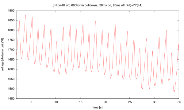
(click to embiggen) Yesterday’s plot with digital low-pass filtering, using y(t) = (x(t) + 7 y(t-1) )/8. There is not much noise, but the baseline wobbles up and down a lot, making the signal hard to process automatically.
Today I decided to brush off my digital filter knowledge, which I haven’t used much lately, and see if I could design a filter using only small integer arithmetic on the Arduino, to clean up the signal more. I decided to use a sampling rate fs = 30Hz on the Arduino, to avoid getting any beating due to 60Hz pickup (not that I’ve seen much with my current setup). The 30Hz choice was made because I do two measurements (IR on and IR off) for each sample, so my actual measurements are at 60Hz, and should be in the same place in any noise waveform that is picked up. (Europeans with 50Hz line frequency would want to use 25Hz as their sampling frequency.)
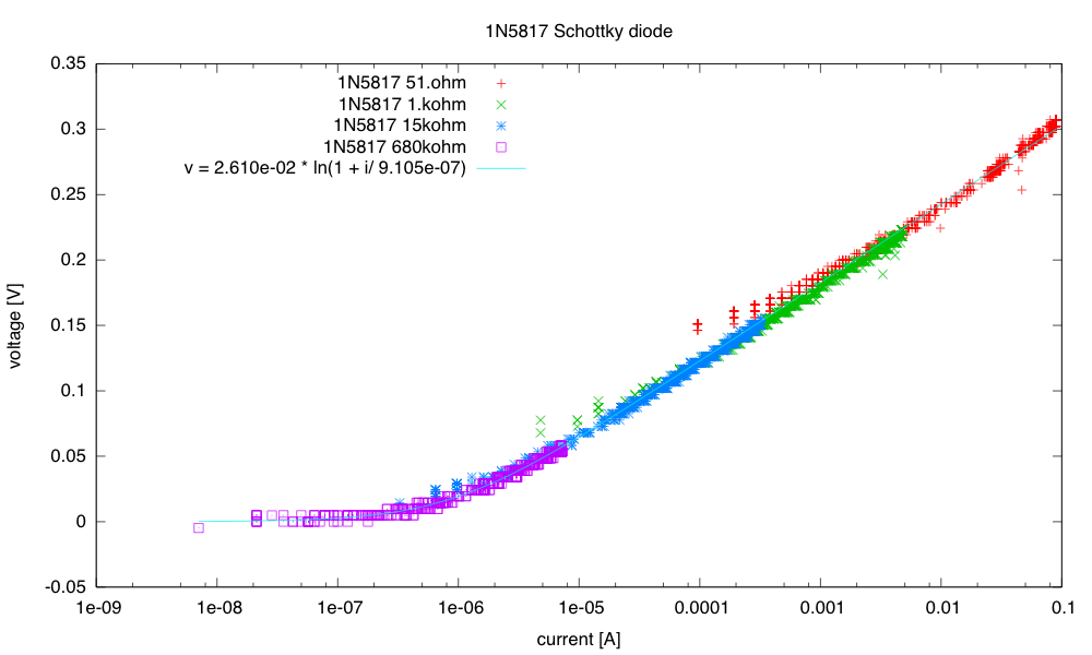
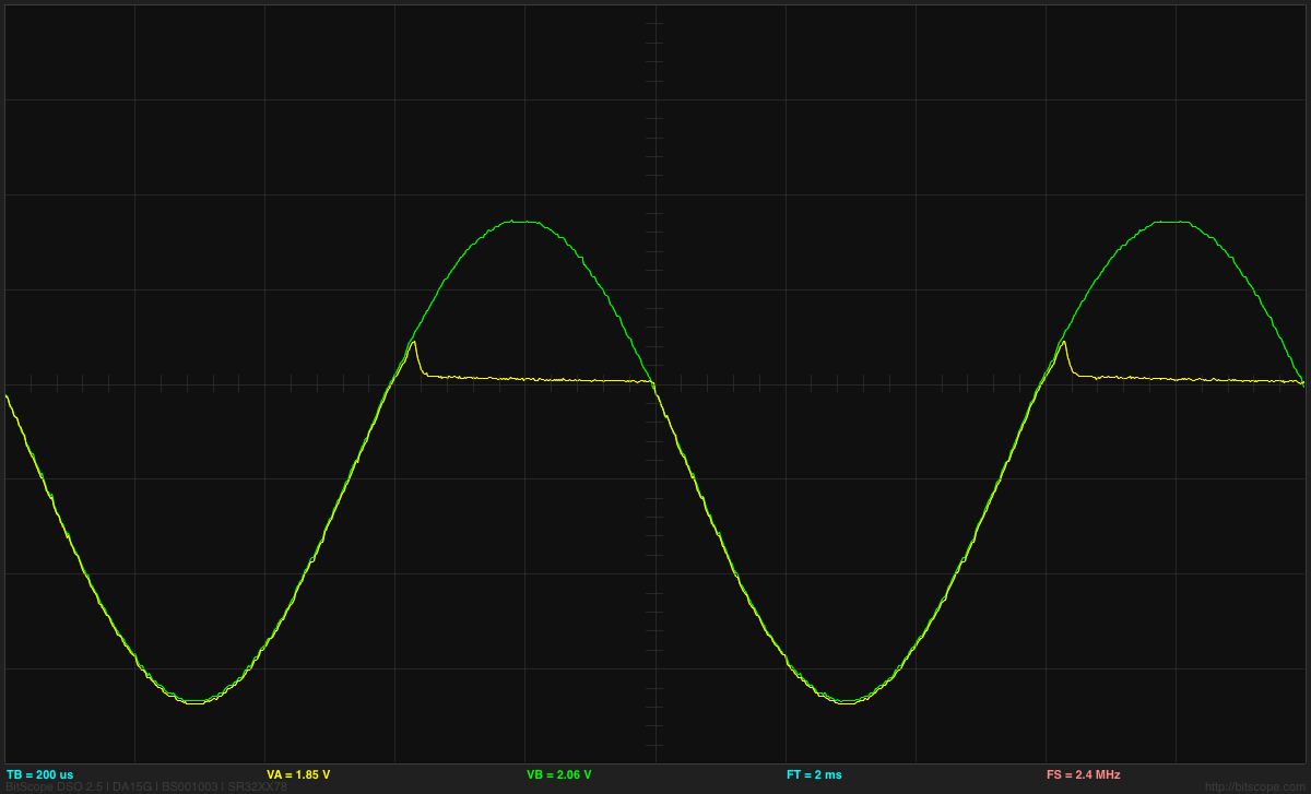
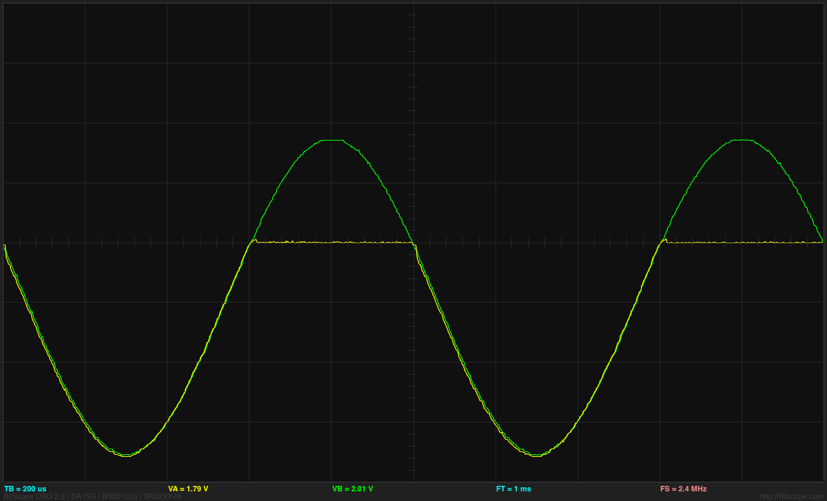
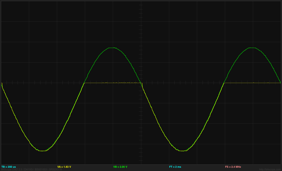
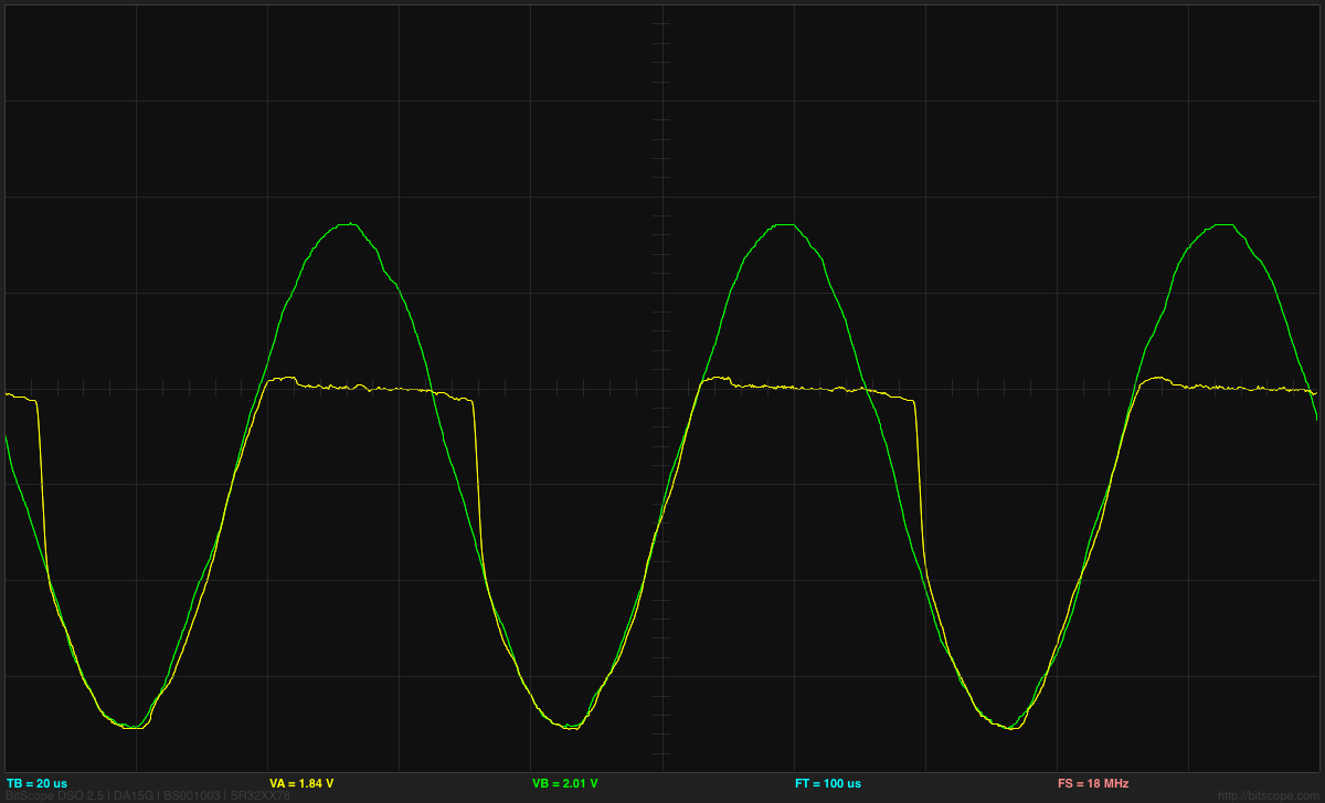
With the 680kΩ resistor that I selected yesterday, the 30Hz sampling leaves plenty of time for the signal to charge and discharge:

The grid line in the center is at 3v. The green trace is the signal to on the positive side of the IR LED, so the LED is on when the trace is low (with 32mA current through the pullup resistor). The yellow trace is the voltage at the Arduino input pin: high when light is visible, low when it is dark. This recording was made with my middle finger between the LED and the phototransistor.
I decided I wanted to replace the low-pass filter with a passband filter, centered near 1Hz (60 beats per minute), but with a range of about 0.4Hz (24 bpm) to 4Hz (240bpm). I don’t need the passband to be particularly flat, so I decided to go with a simple 2-pole, 2-zero filter (called a biquad filter). This filter has the transfer function
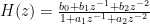
To get the gain of the filter at a frequency f, you just compute  , where
  . Note that the z values that correspond to sinusoids are along the unit circle, from DC at
  up to the Nyquist frequency
  at
at  .
.
The filter is implemented as a simple recurrence relation between the input x and the output y:

This is known as the “direct” implementation. It takes a bit more memory than the “canonical” implementation, but has some nice properties when used with small-word arithmetic—the intermediate values never get any further from 0 than the output and input values, so there is no overflow to worry about in intermediate computations.
I tried using an online web tool to design the filter http://www-users.cs.york.ac.uk/~fisher/mkfilter/, and I got some results but not everything on the page is working. One can’t very well complain to Tony Fisher about the maintenance, since he died in 2000. I tried using the tool at http://digitalfilter.com/enindex.html to look at filter gain, but it has an awkward x-axis (linear instead of logarithmic frequency) and was a bit annoying to use. So I looked at results from Tony Fisher’s program, then used my own gnuplot script to look at the response for filter parameters I was interested in.
The filter program gave me one obvious result (that I should not have needed a program to realize): the two zeros need to be at DC and the Nyquist frequency—that is at ±1. That means that the numerator of the transfer function is just  , and b0=1, b1=0, and b2=–1. The other two parameters it gave me were a2=0.4327386423 and a1=–1.3802466192. Of course, I don’t want to use floating-point arithmetic, but small integer arithmetic, so that the only division I do is by powers of 2 (which the compiler turns into a quick shift operation).
I somewhat arbitrarily selected 32 as my power of 2 to divide by, so that my transfer function is now

and my recurrence relation is

with A1 and A2 restricted to be integers. Rounding the numbers from Fisher’s program suggested A1=-44 and A2=14, but that centered the filter at a bit higher frequency than I liked, so I tweaked the parameters and drew plots to see what the gain function looked like. I made one serious mistake initially—I neglected to check that the two poles were both inside the unit circle (they were real-valued poles, so the check was just applying the quadratic formula). My first design (not the one from Fisher’s program) had one pole outside the unit circle—it looked fine on the plot, but when I implemented it, the values grew until the word size was exceeded, then oscillated all over the place. When I realized what was wrong, I checked the stability criterion and changed the A2 value to make the pole be inside the unit circle.
I eventually ended up with A1=-48 and A2=17, which centered the filter at 1, but did not have as high an upper frequency as I had originally thought I wanted:
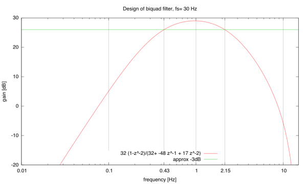
(click to embiggen) The gain of the filter that I ended up implementing has -3dB points at about 0.43 and 2.15 Hz.
Here is the gnuplot script I used to generate the plot—it is not fully automatic (the xtics, for example, are manually set). Click it to expand.
fs = 30	# sampling frequency
A0=32.  # multiplier (use power of 2)
b=16.

A1=-(A0+b)
A2=b+1

peak = fs/A0	# approx frequency of peak of filter

set title sprintf("Design of biquad filter, fs=%3g Hz",fs)

set key bottom center
set ylabel "gain [dB]"
unset logscale y
set yrange [-20:30]

set xlabel "frequency [Hz]"
set logscale x
set xrange [0.01:0.5*fs]

set xtics add (0.43, 2.15)
set grid xtics

j=sqrt(-1)
biquad(zinv,b0,b1,b2,a0,a1,a2) = (b0+zinv*(b1+zinv*b2))/(a0+zinv*(a1+zinv*a2))
gain(f,b0,b1,b2,a0,a1,a2) = abs( biquad(exp(j*2*pi*f/fs),b0,b1,b2,a0,a1,a2))
phase(f,b0,b1,b2,a0,a1,a2) = imag(log( biquad(exp(j*2*pi*f/fs),b0,b1,b2,a0,a1,a2)))

plot 20*log(gain(x,A0,0,-A0,  A0,A1,A2)) \
		title sprintf("%.0f (1-z^-2)/(%.0f+ %.0f z^-1 + %.0f z^-2)", \
			A0, A0, A1, A2), \
	20*log(gain(peak,A0,0,-A0,  A0,A1,A2))-3 title "approx -3dB"
I wrote a simple Arduino program to sample the phototransistor every 1/60th of a second, alternating between IR off and IR on. After each IR-on reading, I output the time, the difference between on and off readings, and the filtered difference. (click on the code box to view it)
#include "TimerOne.h"

#define rLED 3
#define irLED 5

// #define CANONICAL   // use canonical, rather than direct implementation of IIR filter
// Direct implementation seems to avoid overflow better.
// There is probably still a bug in the canonical implementation, as it is quite unstable.

#define fs (30) // sampling frequency in Hz
#define half_period (500000L/fs)  // half the period in usec

#define multiplier  32      // power of 2 near fs
#define a1  (-48)           // -(multiplier+k)
#define a2  (17)            // k+1

volatile uint8_t first_tick;    // Is this the first tick after setup?
void setup(void)
{
    Serial.begin(115200);
//    pinMode(rLED,OUTPUT);
    pinMode(irLED,OUTPUT);
//    digitalWrite(rLED,1);  // Turn RED LED off
    digitalWrite(irLED,1); // Turn IR LED off

    Serial.print("# bandpass IIR filter\n# fs=");
    Serial.print(fs);
    Serial.print(" Hz, period=");
    Serial.print(2*half_period);
    Serial.print(" usec\n#  H(z) = ");
    Serial.print(multiplier);
    Serial.print("(1-z^-2)/(");
    Serial.print(multiplier);
    Serial.print(" + ");
    Serial.print(a1);
    Serial.print("z^-1 + ");
    Serial.print(a2);
    Serial.println("z^-2)");
#ifdef CANONICAL
    Serial.println("# using canonical implementation");
#else
    Serial.println("# using direct implementation");
#endif
    Serial.println("#  microsec raw   filtered");

    first_tick=1;
    Timer1.initialize(half_period);
    Timer1.attachInterrupt(half_period_tick,half_period);
}

#ifdef CANONICAL
// for canonical implementation
 volatile int32_t w_0, w_1, w_2;
#else
// For direct implementation
 volatile int32_t x_1,x_2, y_0,y_1,y_2;
#endif

void loop()
{
}

volatile uint8_t IR_is_on=0;    // current state of IR LED
volatile uint16_t IR_off;       // reading when IR is off (stored until next tick)

void half_period_tick(void)
{
    uint32_t timestamp=micros();

    uint16_t IR_read;
    IR_read = analogRead(0);
    if (!IR_is_on)
    {   IR_off=IR_read;
        digitalWrite(irLED,0); // Turn IR LED on
        IR_is_on = 1;
        return;
    }

    digitalWrite(irLED,1); // Turn IR LED off
    IR_is_on = 0;

    Serial.print(timestamp);
    Serial.print(" ");

    int16_t x_0 = IR_read-IR_off;
    Serial.print(x_0);
    Serial.print(" ");

 #ifdef CANONICAL
    if (first_tick)
    {  // I'm not sure how to initialize w for the first tick
       w_2 = w_1 = multiplier*x_0/ (1+a1+a2);
       first_tick = 0;
    }
 #else
    if (first_tick)
    {   x_2 = x_1 = x_0;
        first_tick = 0;
    }
#endif

#ifdef CANONICAL
    w_0 = multiplier*x_0 - a1*w_1 -a2*w_2;
    int32_t y_0 = w_0 - w_2;
    Serial.println(y_0);
    w_2=w_1;
    w_1=w_0;
#else
     y_0 = multiplier*(x_0-x_2) - a1*y_1 -a2*y_2;
     Serial.println(y_0);
     y_0 /= multiplier;
     x_2 = x_1;
     x_1 = x_0;
     y_2 = y_1;
     y_1 = y_0;
#endif
}
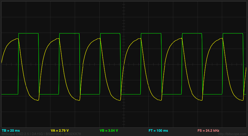
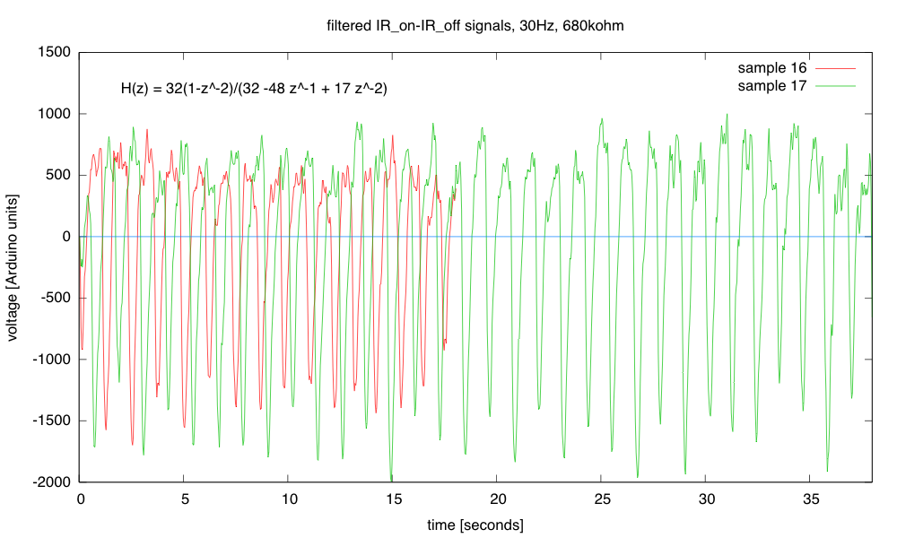
Here are a couple of examples of the input and output of the filtering:

(click to embiggen) The input signals here are fairly clean, but different runs often get quite different amounts of light through the finger, depending on which finger is used and the alignment with the phototransistor. Note that the DC offset shifts over the course of each run.

(click to embiggen) After filtering the DC offset and the baseline shift are gone. The two very different input sequences now have almost the same range. There is a large, clean downward spike at the beginning of each pulse.
Overall, I’m pretty happy with the results of doing digital filtering here. Even a crude 2-zero, 2-pole filter using just integer arithmetic does an excellent job of cleaning up the signal.
Filed under:
Circuits course,
Data acquisition,
freshman design seminar Tagged:
Arduino,
biquad filter,
digital filter,
IIR filter,
IR emitter,
LED,
phototransistor,
pulse,
pulse monitor,
pulse oximeter 


 , where
  . Note that the z values that correspond to sinusoids are along the unit circle, from DC at
  up to the Nyquist frequency
  at
at  .
.
 , and b0=1, b1=0, and b2=–1. The other two parameters it gave me were a2=0.4327386423 and a1=–1.3802466192. Of course, I don’t want to use floating-point arithmetic, but small integer arithmetic, so that the only division I do is by powers of 2 (which the compiler turns into a quick shift operation).


 . Because division is very slow on the Arduino, I limited myself to simple shifts for division: a= 1/2, 1/4, or 1/8. To avoid losing even more precision, I actually output
  then divided by 8 to get Y(t). I also used a 40msec sampling period, with the IR emitter on for 20ms, then off for 20msec (the waveform shown in the oscilloscope trace above).


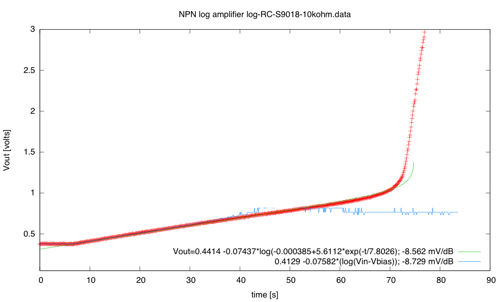
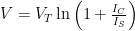
 for some constant x. Note that if we leave the –1 in, then we’ll have a small DC offset to iC.
 is temperature-dependent, since
  , which is about 26mV at 300˚K. The scale factor can be multiplied by ln(10) to get 60mV/decade or 3mv/dB.
 will be poor. If I make R2 small, the current may exceed what the transistor is designed for and there may be saturation effects.

 .
. , and we could make arbitrary tradeoffs between v2 and RC.