Posts with «data acquisition» label

Still more on log amplifiers

Yesterday, I spent the day testing different transistors in the log amplifier, to see whether it made much difference which transistor I used.  I wanted to test all 11 transistors in the iteadstudio assortment, the 5 PNP transistors and the 6 NPN transistors, to see if it made much difference and whether one of the transistors would give me a larger mV/dB scaling than the others.

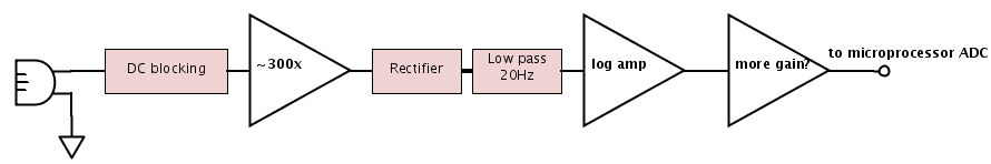
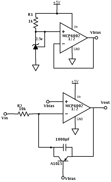
Here is the test circuit I made (essentially the same as for the tests in Logarithmic amplifier again):

(click image to embiggen) The same circuit can be used for either NPN or PNP transistors. The only difference is whether the 470µF capacitor starts at 0v (for PNP) or 5v (for NPN) before decaying to Vbias through the 16kΩ resistor R5. For many of the tests the voltage-to-current resistor R2 was 1kΩ rather than 10kΩ.

The op amp at the top is a unity-gain buffer to provide a steady Vbias source that capable of providing some current (unlike the TL431ILP voltage reference shown here as an adjustable Zener diode). The nominal 2.5V reference was closer to 2.48V, which is within the ±2% spec for the part.

The unity-gain buffer on the left is to make the load on the RC circuit as high impedance as possible, so as not to disrupt the RC charging or discharging. The input current of the MCP6002 is typically ±1pA, which is far smaller than other sources of error (such as the parallel resistance of the capacitor itself). The parallel resistance of the capacitor makes the destination voltage of the RC circuit slightly lower than Vbias, which means that we will not get all the way to Vbias when testing PNP transistors, but will overshoot slightly when testing NPN transistors. (We should be able to reverse that by putting the capacitor between +5V and the switch, rather than ground and the switch.)

The right-hand op amp is just a non-inverting amplifier with 3× gain, to get better precision on measuring the output voltage with the Arduino ADC.  I made some measurements with Vout but most with the 3Vout signal. The scaling factor was 3.0 much more accurately than the repeatability of my fits to the data, so the gain in precision was not accompanied by a loss of accuracy. Ideally, I’d like to be able to use more than a 3× gain in the final stage, to get better precision, but I’m limited by the offset voltage of the log amplifier, which is determined by the transistor and by the voltage-to-current converter R2.

The middle op amp is the log amplifier itself, which relies on the exponential relationship of the emitter current to the voltage across the base-emitter junction. More precisely, we can use the Ebers-Moll model of a bipolar transistor to get

The collector is held at Vbias by the feedback loop of the op amp, so VBC is zero, simplifying the equation to

Assuming that βR and IS are constant, and that VBE is very large compared to VT (about 23 times bigger in my measurements), we have the desired exponential relationship: for some constant x.  Note that if we leave the –1 in, then we’ll have a small DC offset to iC.

(I believe that all this analysis is correct for NPN transistors, where VBE is positive, but that some signs may need to be negated for PNP transistors.)

The log-amplifier output is temperature-dependent, since , which is about 26mV at 300˚K. The scale factor can be multiplied by ln(10) to get 60mV/decade or 3mv/dB.

Note that this scaling is not affected by the current gain β of the transistor—that only affects the offset of the output voltage. This analysis agrees with the statement in Wikipedia, “At room temperature, an increase in VBE by approximately 60 mV increases the emitter current by a factor of 10.” There is probably an even bigger temperature dependence for the offset of the output than for the scaling, because of changes in βR and IS, but that is not included in the Ebers-Moll model.

The theoretical result indicates that I should get about 3mV/dB for any transistor, but that the offset voltage will vary depending on the characteristics of the transistor.  I might also run into effects not included in the Ebers-Moll model, especially at very large or very small collector currents.

Adjusting R2 to change the current can move the output offset around. If I make R2 large and the current small, then VBE will be small, and the approximation will be poor. If I make R2 small, the current may exceed what the transistor is designed for and there may be saturation effects.

Looking at typical collector currents on the I-vs-V plots for the transistors, I’m seeing values like 8–20mA at the high end, so with a 2.5V drop across R2, I want R2 to be at least 300Ω. Initially, I picked 1kΩ, as providing a large current at 2.5V, hoping that this would give a large dynamic range.  Here are a couple of good examples of measurements using the 3× output and R2=1kΩ.

(click image to embiggen) Typical 3× Vout vs Vin curve for a PNP transistor, here the A1015, using R2=1kΩ. This uses Arduino-measured Vin, Vout, and Vbias, so is limited to about 2 decades (40dB).

(click image to embiggen) Typical 3× Vout vs. Vin curve for an NPN transistor, using R2=1kΩ. Again we’re limited by the Arduino ADC to about 40dB of dynamic range.

The exponential decay of the capacitor to about Vbias allows us to extend the range of the fit well past the resolution of the ADC to measure Vin or Vbias. Combining the formulas for the log amplifier and the RC discharge gives us the general formula
.
Fitting the constants for this turns out to be difficult, because v3 is close to zero. If it were exactly zero, the formula would be , and we could make arbitrary tradeoffs between v2 and RC.

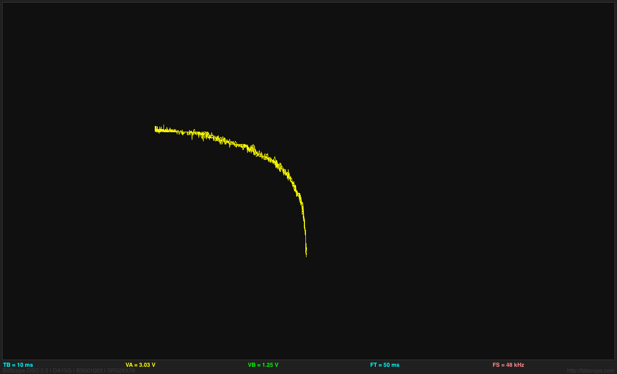
We can get a nice plot of Vout vs. time as the capacitor decays toward Vbias, particularly for the NPN transistor S9013:

(click picture to embiggen) The S9013 log amplifier shows what looks like a good fit over about 80dB, when using R2=1kΩ, and good linearity for about 65dB. The upward tail shows where the collector-base junction begins to be forward biased, and the current is no longer controlled by the base-emitter voltage.

Note that this curve shows that the problems we had with direct measurement of RC discharge curves in the physics lab was due to limitations of the Arduino ADC, not to the underlying RC circuit. The tails of the discharge continue to follow the exponential well beyond the resolution of the 10-bit ADC in the Arduino.

Of course, I picked out the S9013 plot to show, because it was the nicest one. Some of the others were weird. For example, consider the 2N5551:

(click image to embiggen) Not that the 2N5551 Vout vs Vin curve is not a simple logarithm—there is some sort of saturation happening for large input voltages, so the straight-line fit is awful.

The same 2N5551 transistor with R2 at 10kΩ behaves much better:

(click image to embiggen) With a 10kΩ resistor, the currents through the 2N5551 transistor are smaller, and no clipping occurs.

Even weirder was the behavior of the S9018 NPN transistor (the only transistor in the set not matched by a corresponding PNP transistor):

(click image to embiggen) With R2=1kΩ, the S9018 transistor shows a flat spot in the response for  277mV < Vin-Vbias < 330mV (that is, 277uA < IC < 330uA) . I have no idea what causes this flat spot.

I’m still mystified by the flat spot in the S9018 response—anyone have any ideas??

By changing R2 to 10kΩ, we can push the flat spot to 10× higher voltage, just outside the input range that the log amplifier uses:

(click image to embiggen) With R2=10kΩ, the response of the amplifier with a S9018 transistor is nicely logarithmic.

The time response to the RC discharge also looks good:

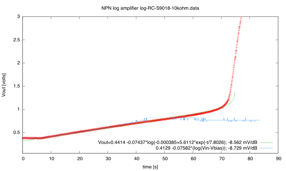
(click to embiggen) With R2=10kΩ, we get a good fit for about 76dB on the S9018 transistor. The larger resistor gives a somewhat softer turn on for the transistor if we go past Vbias.

All of my transistors gave mV/dB scaling that was about the same (just under 9 mV/dB after the 3× gain, so just under 3mV/dB for the unamplified output), as is predicted by the Ebers-Moll model.  I got better dynamic ranges for the NPN transistors than for the PNP transistors, but this may have been due to artifacts of the test setup.  In any case, it looks like 60–70dB ranges are fairly easily achieved.

[UPDATE 2013 July 15: I know I said I was done with the log amplifiers, but I had to do just one more test.  In addition to the 16kΩ resistor to Vbias, I added a 5.7MΩ resistor to +5V, giving me a slightly higher target voltage so that I had some overshoot when testing PNP transistors.  With this setup I could test the S9012 PNP transistor for 82dB with R2=1kΩ, and 63dB with R2=10kΩ.  So the better dynamic range of the NPN was just an artifact of my test setup, as I thought.]

If one were to try to make a measuring instrument with a log amplifier, there would have to be some temperature compensation as the log-amplifier offset and scaling are both temperature sensitive.  Having a temperature-independent voltage source for calibration would be a good idea.

I think I’m about burned out on log amplifiers now.  Perhaps later his week I’ll try doing some precision rectifier circuits.


Filed under: Circuits course, Data acquisition Tagged: Arduino, bipolar transistors, i-vs-v-plot, log amplifier, op amp

Logarithmic amplifier again

Yesterday, in Logarithmic amplifier, I ended with the following plot:

(click plot to see larger version) The cloud of points is broad enough to be consistent with slightly different parameter values.

I was bothered by the broad cloud of points, and wanted to come up with a better test circuit—one that would give me more confidence in the parameters.  It was also quite difficult to get close to Vbias—the closest this could measure was one least-significant-bit of the DAC away (about 5mV).  A factor of 512 from the largest to the smallest signal is 54dB, but only about the upper 40dB of that was good enough data for fitting (and very little time was spent at near the Vbias value).

I think that part of the problem with the cloud was that the input signal was changing fairly quickly, and the Arduino serializes its ADC, so that the input and output are measured about 120µsec apart.  I decided to use a very simple slow-changing signal: a capacitor charging toward Vbias through a large resistor.  My first attempt used a 1MΩ resistor and a 10µF capacitor, for a 10-second time constant:

Output voltage from log amplifier (with 3x gain in second stage) as capacitor charges. (click picture for larger version) One fit uses the Arduino-measured Vin and Vbias voltages, the other attempts to model the RC charging as well. What are the weird glitches?

The capacitor charging should be a smooth curve exponential decay to Vbias, so the log amplifier output should be a straight line with time. There were two obvious problems with this first data—the output was not a straight line and there were weird glitches about every 15–20 seconds.

The non-straight curve comes from the capacitor not charging to Vbias. Even when the capacitor was given lots of time to charge, it remained stubbornly below the desired voltage. In think that the problem is leakage current: resistance in parallel with the capacitor. The voltage was about 1% lower than expected, which would be equivalent to having a 100MΩ resistor in parallel with the capacitor.  I can well believe that I have sneak paths with that sort of resistance on the breadboard as well as in the capacitor.

According to Cornell Dublier, a capacitor manufacturer, a typical parallel resistance for a 10µF aluminum electrolytic capacitor would be about 10MΩ [http://www.cde.com/catalogs/AEappGUIDE.pdf‎]:

Typical values are on the order of 100/C MΩ with C in μF, e.g. a 100 μF capacitor would have an Rp of about 1 MΩ.

So I may be lucky that I got as close to Vbias as I did.

The glitches had a different explanation: they were not glitches in the log amplifier circuit, but in the 5V power supply being used as a reference for the ADC on the Arduino board—I had forgotten how bad the USB power is coming out of my laptop, though I had certainly observed the 5V supply dropping for a second about every 20 seconds on previous projects.  The drop in the reference for the ADC results in a bogus increase in the measured voltages.  That problem was easy to fix: I plugged in the power supply for the Arduino rather than running off the USB power, so I had a very steady voltage source using the Arduino’s on-board regulator.

(click picture for larger version) With a proper power supply, I get a clean charge and the output is initially a straight line, but I’m still not getting close to Vbias. Again the blue fit uses the measured Vin and Vbias voltages, while the green curve tries to fit an RC decay model. Note the digitization noise on the measured inputs towards the end of the charging time.

To solve the problem of the leakage currents, I tried going to a larger capacitor and smaller resistor to get a similar RC time constant. At that point I had not found and read the Cornell Dublier application note, though I suspected that the parallel resistance might scale inversely with the capacitor size, in which case I would be facing the same problem no matter how I chose the R-vs-C tradeoff. Only reducing the RC time constant would work for getting me closer to Vbias.

Using a 47kΩ resistor and a 470µF capacitor worked a bit better, but the time constant was so long that I got impatient:

(click image for larger version) The blue fit is again using the measured Vin and Vbias, and has a pretty good fit. The green fit using an RC charge model does not seem quite as good a fit.

The calibration of 9.7mV/dB seems pretty good, so the 409mV range of the recording corresponds to a 42dB range. The line is straighter, but I’m still not getting as close to Vbias as I’d like.

I then tried a smaller RC time constant (hoping that the larger current with the same capacitor would result in getting closer to Vbias, and so testing a larger dynamic range on the log amplifier). I tried 16kΩ with the 470µF capacitor:

(click image to embiggen) I’m now getting a clear signal from the log amplifier even after the input voltage has gotten less than one least-significant-bit away from Vbias (the blue fit). I found it difficult to fit parameters for modeling the RC charge (the green fit).

The two models I fit to the data give me somewhat different mV/dB scales, though both fit the data fairly well. The blue curve fits better up to about 65 seconds, then has quantization problems. Using that estimate of 9.8mV/dB and the 560mV range of the output, we have a dynamic range here of 57dB. There is still some flattening of the curve—we aren’t quite getting to the Vbias value, but it is pretty straight for the first 50 seconds.

Note: the parallel resistance of the capacitors would not explain the not-quite-exponential behavior we saw in the RC time constant lab, since those measurements were discharging the capacitor to zero. A parallel resistance would just change the time constant, not the final voltage.

I was using the Duemilanove board for the log-amplifier tests. I retried with the Uno board, to see if differences in the ADC linearity make a difference in the fit:

(click to embiggen) Using the Uno Arduino board I still had trouble with the fit, and the Uno ADC seems to be noisier than the Duemilanove ADC. The missing parts of the blue curve are where the Uno board read the input as having passed Vbias.

The 625 mV range over 250 seconds corresponds to about 69dB, assuming that the 9.1 mV/dB calibration is reasonably accurate (and 64dB if the earlier 9.8mV/dB calibration is better).
My measurements of the log amplifier do not seem to yield a very consistent mV/dB parameter, with values from 9.1mV/dB to 9.8mV/dB using just the Arduino measurements (and even less consistency when a model of RC charging is used).  I’m not sure how I can do more consistent measurements with the equipment I have.  Anyone have any ideas?
Incidentally, my son has decided not to include a microphone in his project.  The silicon MEMS mic was small enough, but the op amp chip for the analog processing was too big for the small board area he had left in his layout, and he decided that the loudness detector was not valuable enough for the board area and parts cost. I believe that his available board area shrunk a little today, because he discovered that the keep-away check had not been turned on in the Eagle design-rule checker.  Turning it on indicated that he had packed the capacitors too close in places, and he had to spread them out. (At least, I think that’s what he told me—I’ve not been following his PC board layout very closely.)
I’m still interested in learning about log amplifiers and precision rectifiers, so I’m still going to breadboard the components of the design and test them out.  I’m not sure when I’ll ever use the knowledge, since the Applied Circuits course does not cover the nonlinear behavior of pn junctions nor the forward-voltage drop of diodes (we don’t use diodes in the course).


Filed under: Circuits course, Data acquisition Tagged: Arduino, BitScope, i-vs-v-plot, log amplifier, loudness, op amp

Logarithmic amplifier

My son wanted to design a circuit to convert microphone inputs to loudness measurements usable by an Arduino (or other ATMega processor).  We discussed the idea together, coming up with a few different ideas.

The simplest approach would be to amplify the microphone then do everything digitally on the Arduino. There are several features of this approach:

  • The analog circuit is about as simple as we can get: a DC-blocking capacitor and an amplifier.  This would only need one op amp, one capacitor, and 2 resistors (plus something to generate a bias voltage—perhaps another op amp, perhaps a low-drop-out regulator).
  • Using digital processing, he can do true RMS voltage computation, and whatever low-pass filtering to smooth the result that he wants.
  • He can’t sample very fast on the ATMega processor, so high frequencies would not be handled properly.  He might be able to sample at 9kHz (about as fast as the ADC operates), but that limits him to 4.5kHz. For his application, that might be good enough, so this doesn’t kill the idea.
  • He’d like to have a 60dB dynamic range (say from 50dB to 110dB) or more, but the ADC in the ATMega is only a 10-bit converter, so a 60dB range would require the smallest signal to be ±½LSB, which is at the level of the quantization noise.  With careful setting of the gain for the microphone preamp, one might be able to get 55dB dynamic range, but that is pushing it a bit.  The resolution would be very good at maximum amplitude, but very poor for quiet inputs.

Although the mostly digital solution has not been completely ruled out, he wanted to know what was possible with analog circuits.  We looked at two main choices:

  • True-RMS converter chips (intended for multimeters).  These do all the analog magic to convert an AC signal to a DC signal with the same RMS voltage.  Unfortunately, they are expensive (over $5 in 100s) and need at least a 5v power supply (he is planning to use all 3.3v devices in his design).  Also true RMS is a bit of overkill for his design, as log(amplitude) would be good enough.
  • Using op amps and discrete components to make an amplifier whose output is the logarithm of the amplitude of the input.  Together we came up with the following block diagram:

Block diagram of the loudness circuit. (drawn with SchemeIt).

We then spent some time reading on the web how to make good rectifier circuits and logarithmic amplifiers. I’ll do a post later about the rectifier circuits, since there are many variants, but I was most interested in the logarithmic amplifier circuits, which rely on the exponential relationship between current and voltage on a pn junction—often the emitter-base junction of a bipolar transistor.

My son wanted to know what the output range of the log amplifier would be and whether he would need another stage of amplification after the log amplifier. Unfortunately, the theory of the log amplifier uses the Shockley ideal diode equation, which needs the saturation current of the pn junction—not something that is reported for transistors.  There is also a “non-ideality” parameter, that can only be set empirically.  So we couldn’t compute what the output range would be for a log amplifier.

Today I decided to build a log amplifier and see if I could measure the output.  I also wanted to figure out what sort of dynamic range he could get from a log amp. Here is the circuit I ended up with, after some tweaking of parameters:

The top circuit is just a bias voltage generator to create a reference voltage from a single supply. I’m working off of 5v USB power, so I set the reference to 2.5v. He might want to use a 1.65v reference, if he is using 3.3v power.
The bottom circuit is the log amplifier itself.

I chose a PNP transistor so that Vout would be more positive as the input current got further from Vbias.  I have 6 different PNP transistors from the Iteadstudio assortment of 11 different transistors, and I chose the A1015 rather arbitrarily, because it had the lowest current gain. I should probably try each of the other PNP transistors in this circuit, to see how sensitive the circuit is to the transistor characteristics.  I suspect it is very sensitive to them.

The circuit only works if the collector-base junction is reverse-biased (the usual case for bipolar transistors), so that the collector current is determined by the base current. The emitter-base junction may be either forward or reverse biased.  Note that if Vin is larger than Vbias, the collector-base junction becomes forward-biased, the negative input of the op amp is slightly above Vbias, and the op amp output hits the bottom rail.

As long as Vin stays below Vbias, the current through R2 should be , and the output voltage should be for some constants A and B that depend on the transistor. Note that changing R2 just changes the offset of the output, not the scaling, so the range of the output is not adjustable without a subsequent amplifier.

The 1000pF capacitor across the transistor was not part of the designs I saw on the web, but I needed to add it to suppress high-frequency (around 3MHz) oscillations that occurred. The oscillations were strongest when the current through R2 was large, and the log output high.  I first tried adding a base-emitter capacitor, which eliminated the oscillations, but I still has some lower-frequency oscillations when the transistor was shutting off (very low currents).  Moving the capacitor to be across the whole transistor as shown in the schematic cleaned up both problems.

I put ramp and sine wave inputs into the log amplifier.  The waveforms were generated with the Bitscope function generator, which does not allow setting the offset very precisely—there is only an 8-bit DAC generating the waveform.  Here is a sample waveform:

Click picture for larger image. The green trace is the input, the yellow trace is the output. The horizontal axis in the middle is at 2.5V for the input (so the input is always below 2.5V) and at 3V for the output. The scale is 1V/division for the input and 50mV/division for the output.  [And all those values should be visible in the saved snapshot, but they aren't.]

The ripple on the output is mainly artifacts of the low-resolution of the BitScope A-to-D converter—smoothing of multiple reads is done, but there is a lot of quantization noise. According to my analog scope there are still some 24MHz noise around, but it seems to be from the Vbias source—adding a 4.7µF capacitor between Vbias and +5V (adjacent pins on the op amp) cleaned things up a lot on the analog scope, without affecting the BitScope traces.

Using the cursors on the BitScope, I was able to measure the output voltages for input voltages of Vbias-0.5V, Vbias-1V, and Vbias-2.5V.  From these, I concluded that the scaling factor for the output was about 3.1–3.2 mv/dB.  The output was 3±0.07V, so the dynamic range is 140mV/(3.2 mv/dB), or about 44dB.  We can see the logarithmic response in an X-Y plot of the output vs the input:

(Click for larger image) Output vs. input of the log amplifier. Note that the output is the log of Vbias-Vin, so the log curve looks backwards here.  It’s a shame that BitScope throws away the grid on XY plots, as the axes are still meaningful.

I also tried using an external oscillator, so that I could get better control of the offset voltage, and thus (perhaps) a better view of the dynamic range. I could fairly reliably get an output range of about 200mV, without the hysteresis that occurs when the collector-base junction gets forward biased. That would be over 60dB of dynamic range, which should be fine.

I should be able to adjust the voltage offset of the amplifier by changing R2. Increasing R2 reduces the current, which should lower the voltage. I tried several different values for R2 and measured the maximum output voltage, using the same input throughout:

1kΩ 3.106v
10kΩ 3.056v
100kΩ 2.992v
1MΩ 2.936v

The 60dB difference in current produces a 170mV difference in output, for 2.83 mV/dB.

Oops, those weren’t quite all the same, as the load from the resistor changes the input. Adding a unity-gain buffer driving the inputs and adjusting the input so that the output of the unity gain buffer has a slight flat spot at 0V gives me a new table:

1kΩ 3.12v
10kΩ 3.06v
100kΩ 3.00v
1MΩ 2.94v
5.6MΩ 2.90v

which is consistent with 3mV/dB. I was not able to extend this to lower resistances, as I started seeing limitations on the output current of the op amp. But it is clear that the amplifier can handle a 75dB range of current, with pretty good log response.

An Arduino input is about 5mV/count, so the resolution feeding the output of the log amplifier directly into the Arduino would be about 1.7dB/count. We could use a gain of 4 without saturating an op amp (assuming that we use 2.5V as the center voltage still), for about a 0.4 dB resolution. More reasonably, we could use a gain of 3 to get a resolution of about 0.54dB/count.

I tried that, getting the following table:

1kΩ 4.46v
10kΩ 4.28v
100kΩ 4.10v
1MΩ 3.91v
5.6MΩ 3.78v

This table is consistent with 9.1 mv/dB, for a resolution of about 0.54 dB/step on the Arduino.

I tried using the Arduino to collect the same data and fit with gnuplot:

(click plot to see larger version) The gnuplot fit agrees fairly well with the measurements made with the BitScope for 5 resistor values. The resolution of the Arduino DAC limits the ability to measure the dynamic range, and the cloud of points is broad enough to be consistent with slightly different parameter values.

The next thing for me to do on the log amp is probably to try different PNP transistors, to see how that changes the characteristics. My son will probably want to use a surface-mount transistor, so we’ll have to find one that is also available as a through-hole part, so that we can check the log amplifier calibration.


Filed under: Data acquisition Tagged: Arduino, BitScope, i-vs-v-plot, log amplifier, loudness, op amp

Pressure sensor with air pump

I’ve been thinking of expanding the pressure sensor lab for the Applied Circuits Course to do something more than just measure breath pressure.  Perhaps something that conveys another physics or engineering concept.

One thing I thought of doing was measuring the back pressure and air flow on an aquarium air pump bubbling air into an aquarium. Looking at the tradeoff of flow-rate and back pressure would be a good characterization of an air pump (something I wish was clearly shown in advertisements for aquarium air pumps and air stones).  Measuring flow rate is a bit of a pain—about the best I could think of was to bubble air into an inverted soda bottle (or other known volume) and time it.

This would be a good physics experiment and might even make a decent middle-school product-science science fair project (using a cheap mechanical low-pressure gauge, rather than an electronic pressure sensor), but setting up tanks of water in an electronics lab is a logistic nightmare, and I don’t think I want to go there.

I can generate back pressure with just a simple clamp on the hose, though, and without a flow rate measurement we could do everything completely dry.

Setup for measuring the back pressure for an aquarium air pump (needs USB connection for data logger and power).

Using the Arduino data loggger my son wrote, I recorded the air pressure while adjusting the clamp (to get the y-axis scale correct, I had to use the estimated gain of the amplifier based on resistor sizes used in the amplifier).

The peak pressure, with the clamp sealing the hose shut, seems to be about 14.5 kPa (2.1psi).

I was interested in the fluctuation in the pressure, so I set the clamp to get about half the maximum back pressure, then recorded with the Arduino data logger set to its highest sampling frequency (1ms/sample).

The fluctuation in back pressure seems to have both a 60Hz and a 420Hz component with back pressure at about half maximum.

Because the Arduino data logger has trouble dealing with audio frequency signals, I decided to take another look at the signals using the Bitscope pocket analyzer.

The waveform for the pressure fluctuations from the AQT3001 air pump, with the back pressure about 7.5kPa (half the maximum).

One advantage of using the Bitscope is that it has FFT analysis:

Spectrum for the back pressure fluctuation. One can see many of the multiples of 60Hz, with the particularly strong peak at 420Hz.

I was also interested in testing a Whisper40 air pump (a more powerful, but quieter, pump). When I clamped the hose shut for that air pump, the hi-gain output of the amplifier for the pressure sensor saturated, so I had to use the low gain output to determine the maximum pressure (24.8kPA, or about 3.6psi). The cheap Grafco clamp that I used is a bit hard to get complete shutoff with (I needed to adjust the position of the tubing and use pliers to turn the knob).  It is easy to get complete shutoff if the tube is folded over, but then modulation of less than complete shutoff is difficult.

The fluctuation in pressure shows a different waveform from the AQT3001:

The Whisper40 air pump, with the clamp set to get a bit less than half the maximum back pressure, produces a 60Hz sawtooth pressure waveform, without the strong 420Hz component seen from the AQT3001. The peak-to-peak fluctuation in pressure seems to be largest around this back pressure. The 3kPa fluctuation is larger than for the AQT3001, but the pump seems quieter.

The main noise from the pump is not from the fluctuation in the pressure in the air hose, but radiation from the case of the pump. That noise seems to be least when the back pressure is about 1.1kPa (not at zero, surprisingly). The fluctuation is then all positive pressure, ranging from 0 to 2.2kPa and is nearly sinusoidal, with some 2nd and 3rd harmonic.

As the back pressure increases for the Whisper40, the 2nd, 3rd, and 4th harmonics get larger, but the 60Hz fundamental gets smaller. The 4th harmonic is maximized (with the 1st through 4th harmonics almost equal) at about 22.8kPa, above which all harmonics get smaller, until the air hose is completely pinched off and there is no pressure variation.

When driving the large airstone in our aquarium, the Whisper40 has a back pressure of about 7.50kPa (1.1psi) with a peak-to-peak fluctuation of about 2.6kPa.

I’m not sure whether this air-pump back-pressure experiment is worth adding to the pressure sensor lab.  If I decide to do it, we would need to get a dozen cheap air pumps.  The Tetra 77853 Whisper 40 air pump is $11.83 each from Amazon, but the smaller one for 10-gallon aquariums is only $6.88.  With 12 Ts and 12 clamps, this would cost about $108, which is not a significant cost for the lab.


Filed under: Circuits course, Data acquisition, Pressure gauge Tagged: air pump, Arduino, BitScope, circuits, data acquisition, data logger, instrumentation amp, oscilloscope, pressure sensor, science fair, USB oscilloscope

Arduino data logger at Global Physics Department

My son presented the Arduino Data Logger he wrote for my circuits class to the Global Physics Department on 2013 May 15.  The sessions are recorded, and the recording is available on the web (though you have to run Blackboard Collaborate through Java Web Start to play the recording).

I thought he did a pretty good job of presenting the features of the data logger.

Now that school is beginning to wind down, he’s started looking at making modifications to the data logger code again, and has updated it at https://bitbucket.org/abe_k/arduino-data-logger/

He’s down to only three classes now (US History, Physics, and Dinosaur Prom Improv), though he still has homework to catch up on in Dramatic Literature and his English class.  He’s still TAing for the Python class also.

On Thursday and Friday this week, he’ll be taking the AP Computer Science test and the AP Physics C: Electricity and Magnetism test.  He’s having to take both tests in the “make-up” time slot, because we couldn’t get any local high school to agree to proctor the tests for him during the regular testing time.  Eventually his consultant teacher convinced the AP coordinator to let her proctor the tests, but by then it was too late to register for anything but the makeup tests. We’re way behind schedule on the physics class, so he’s just going to read the rest of the physics book without working any problems before Friday’s exam—we’ll finish the book in a more leisurely fashion after the exam. He won’t be as prepared for the physics exam as I had hoped, but at least the CS exam looks pretty easy to him.

One thing I didn’t realize is that schools can charge homeschoolers whatever the market will bear for proctoring the tests:

  • Depending on the reasons for late testing, schools may be charged an additional fee ($40 per exam), part or all of which the school may ask students to pay. Students eligible for the College Board fee reduction will not be charged the $40-per-exam late-testing fee, regardless of their reason for testing late.
  • Schools administering exams to homeschooled students or students from other schools may negotiate a higher fee to recover the additional proctoring and administration costs.

[ http://professionals.collegeboard.com/testing/ap/about/fees ]

We’re paying $145 per exam (not just the $89 standard fee and the $40 late fee), but I’m glad he gets to take the exams at all this year.

Tomorrow he and I are doing another campus tour—this time at Stanford. He managed to get an appointment with a faculty member, but we noticed that the faculty member is scheduled to be teaching a class at the time of the appointment—I wonder what is going to happen with that. I’ll report on the visit later this week.


Filed under: Data acquisition Tagged: Advanced Placement exams, Arduino, data logger, Global Physics Department, physics

Data logging software for circuits course working

Over winter break, my son has been working nearly full time on writing data logging software for my students to use in the Applied Circuits for Bioengineers course. He has made the first public beta release (v1.0.0b1) today on BitBucket. (Note: you may have to click on the “tags” tab to get to the view that shows the v1.0.0b1 link. The BitBucket link directly to that view seems to be broken—that’s open issue 5504 in BitBucket’s own issue tracker.)

We’ve only tested the code on Mac OS X computers with Arduino Duemilanove and Uno boards, though we’ve tested a slightly earlier version on Windows.  The code should also run on Linux and with Leonardo and Mega boards, but has not been tested on these platforms. We welcome users testing the code for us—report any problems using the BitBucket issue tracker for the project.  The documentation is still in a fairly primitive state—report issues with that also, so that they can be fixed.

The overall goal is fairly simple: to have an easy-to-use way to record timestamps, voltages, and digital values from the Arduino into files on a host computer, without needing auxiliary hardware (like the Adafruit data logger shield that I bought for myself and assembled yesterday).

The user can specify what analog and digital pins to record and when to record the values.  When to record can be specified either   as interrupts on pins or as fixed timing intervals:

View of the two windows of the user interface.

The “volts measured” for the reference is stored as metadata in the output file and can be used for scaling the Arduino numbers (if “Convert to Volts” is checked).  The scaling can be an arbitrary value for the full-scale reading or can be the voltage measured with an external multimeter at the AREF pin.

This software has been through several versions:

  1. The first version of the code was one I wrote last spring that just recorded interrupt times in an Arduino array and dumped them out over the USB cable after it was done (see Homemade super pulley).
  2. My son was not happy with that crude program of mine and rewrote it in June to have use the Arduino memory as a queue and send the time stamps to a Python program on the laptop (see Improved super pulley code).  That program introduced him to three new concepts: circular buffers for queues, interrupts, and multi-threading, all of which he researched for himself. That version of the code mainly used a command line interface, but he used the curses package for a crude user interface.
  3. He added a PyGUI graphical user interface, but that slowed down the code on the laptop and eventually grew to be difficult to maintain.
  4. He decided to try to make the software by portable between three platforms (Mac OS X, Windows, and Linux) despite their very different ways of dealing with the USB serial ports, to run under both Python2.7 and Python3, and to require only minimal non-standard packages (mainly PySerial and the Arduino package Timer1).  He refactored the code completely and built the GUI using Tkinter. This has lead to the current version of the code, which is finally working robustly enough to let the bioengineering students use it.

It has been a good software-engineering experience for my son, and he has learned a lot.  In the process of developing this code, he has learned a lot about interrupts, using queues to communicate between processors and between threads, platform-independence, a couple of different GUI libraries, the value of version control and bug-tracking, race conditions, interface design for non-expert users, and even some things about documentation.

I’ve been acting mainly as a customer for this code, entering bug reports and suggesting new features, though I have occasionally helped him debug.  For example, we just spent fifteen minutes reading Section 15 “16-bit Timer/Counter1 with PWM” of the ATMega328 data sheet, trying to figure out why the first time interval was wrong.  It turns out that timer interrupt is raised immediately when the interrupt is enabled, unless the timer-overflow flag is turned off first.

My son may use this project as a science fair entry this year, though it was not started with that idea, and we discussed that possibility for the first time today.  The big problem is that this is purely an engineering project, not a “science” project, and trying to fake a hypothesis is not something we’ll consider.


Filed under: Circuits course, Data acquisition, home school, Science fair Tagged: Arduino, bioengineering, BitBucket, circuits, data logger