Over winter break, my son has been working nearly full time on writing data logging software for my students to use in the Applied Circuits for Bioengineers course. He has made the first public beta release (v1.0.0b1) today on BitBucket. (Note: you may have to click on the “tags” tab to get to the view that shows the v1.0.0b1 link. The BitBucket link directly to that view seems to be broken—that’s open issue 5504 in BitBucket’s own issue tracker.)

We’ve only tested the code on Mac OS X computers with Arduino Duemilanove and Uno boards, though we’ve tested a slightly earlier version on Windows.  The code should also run on Linux and with Leonardo and Mega boards, but has not been tested on these platforms. We welcome users testing the code for us—report any problems using the BitBucket issue tracker for the project.  The documentation is still in a fairly primitive state—report issues with that also, so that they can be fixed.

The overall goal is fairly simple: to have an easy-to-use way to record timestamps, voltages, and digital values from the Arduino into files on a host computer, without needing auxiliary hardware (like the Adafruit data logger shield that I bought for myself and assembled yesterday).

The user can specify what analog and digital pins to record and when to record the values.  When to record can be specified either   as interrupts on pins or as fixed timing intervals:

View of the two windows of the user interface.

The “volts measured” for the reference is stored as metadata in the output file and can be used for scaling the Arduino numbers (if “Convert to Volts” is checked).  The scaling can be an arbitrary value for the full-scale reading or can be the voltage measured with an external multimeter at the AREF pin.

This software has been through several versions:

1. The first version of the code was one I wrote last spring that just recorded interrupt times in an Arduino array and dumped them out over the USB cable after it was done (see Homemade super pulley).
2. My son was not happy with that crude program of mine and rewrote it in June to have use the Arduino memory as a queue and send the time stamps to a Python program on the laptop (see Improved super pulley code).  That program introduced him to three new concepts: circular buffers for queues, interrupts, and multi-threading, all of which he researched for himself. That version of the code mainly used a command line interface, but he used the curses package for a crude user interface.
3. He added a PyGUI graphical user interface, but that slowed down the code on the laptop and eventually grew to be difficult to maintain.
4. He decided to try to make the software by portable between three platforms (Mac OS X, Windows, and Linux) despite their very different ways of dealing with the USB serial ports, to run under both Python2.7 and Python3, and to require only minimal non-standard packages (mainly PySerial and the Arduino package Timer1).  He refactored the code completely and built the GUI using Tkinter. This has lead to the current version of the code, which is finally working robustly enough to let the bioengineering students use it.

It has been a good software-engineering experience for my son, and he has learned a lot.  In the process of developing this code, he has learned a lot about interrupts, using queues to communicate between processors and between threads, platform-independence, a couple of different GUI libraries, the value of version control and bug-tracking, race conditions, interface design for non-expert users, and even some things about documentation.

I’ve been acting mainly as a customer for this code, entering bug reports and suggesting new features, though I have occasionally helped him debug.  For example, we just spent fifteen minutes reading Section 15 “16-bit Timer/Counter1 with PWM” of the ATMega328 data sheet, trying to figure out why the first time interval was wrong.  It turns out that timer interrupt is raised immediately when the interrupt is enabled, unless the timer-overflow flag is turned off first.

My son may use this project as a science fair entry this year, though it was not started with that idea, and we discussed that possibility for the first time today.  The big problem is that this is purely an engineering project, not a “science” project, and trying to fake a hypothesis is not something we’ll consider.

My son and I bicycled up to campus today to test out his data logger code (that will be used in the circuits course) on the Windows computers in the lab.  The lab support staff had told me yesterday that they had gotten Python 2.7.3 installed and the Arduino 1.0.3 development environment, as well as the PySerial module that the data logger code requires.

My son has been working pretty intensely on the code lately, doing a complete refactoring of the code to use TKinter (instead of PyGUI, which is difficult to install and quite slow) and to have a more user-friendly GUI.  He also wanted to make the code platform independent (Windows, Mac, and Linux), though he’d only tested on our Macs at home before today.  He’s also trying to make the Python part of the code (the user interface) work in both Python 2.7.3 and Python 3.3, though the languages are not precisely compatible.

We found three problems today:

1. Python 2.7.3 was not quite completely installed.  They’d forgotten to update the path to include C:\Python27\  (The path should also include where the Arduino software was installed—I forget where that was now.)
2. The device drivers for the Arduinos were not installed.  On Macs, there are no drivers to install, but on Windows, you need different drivers for different Arduino boards, and it seems you need to have the board plugged into the USB port in order to install the drivers. (Instructions at http://arduino.cc/en/Guide/Windows#t0c4)
3. My son had forgotten to include one of the dependencies in his list of what needed to be installed—the Arduino Timer1 module from http://playground.arduino.cc/code/Timer1/ .

Because they had given me administrator privileges on the machines, my son was able to fix one of the machines to run the data logger code (though he had a couple of minor changes to make in his code for Windows compatibility also).

For the data logger debugging, about all I did was type in my password for him, and once do a search to see where the Arduino code was hidden.

When he has finished debugging and documenting the code, my son will be releasing it with a permissive license on bitbucket, and I’ll be putting links to it here and on the course web page.

I had a good discussion with Steve P. this afternoon about the order and purpose of the labs I’ve designed so far.  He’ll be putting together a list of EE topics we have to cover to coordinate with the labs, so that students will have enough theory to do each lab, but not be overwhelmed with theory that they don’t yet have a use for.

I’ve designed the labs mainly around the interests of bioengineering majors, but I’ve tried to keep in mind other possible students, such as Digital Arts and New Media students, who would be interested in practical sensor circuits for interfacing to art projects (particularly for inputs to Arduino microprocessors).

Lab 1: thermistor

See posts

1. More musings on circuits course: temperature lab
2. Temperature lab, part2
3. Temperature lab, part 3: voltage divider

The first lab will consist of 3 parts, all involving the use of a Vishay BC Components NTCLE413E2103F520L thermistor.

First, the students would use a bench multimeter to measure the resistance of the thermistor, dunking it in various water baths (with thermometers in them to measure the temperature).  They should fit a simple curve to this data (warning: temperature needs to be on an absolute scale).

Second, they would add a series resistor to make a voltage divider. They have to choose a value to get as large and linear a voltage response as possible at some specified “most-interesting” temperature (perhaps body temperature, perhaps room temperature, perhaps DNA melting temperature).  There should probably be a pre-lab exercise where they derive the formula for maximizing . They would then measure and plot the voltage output for the same set of water baths. If they do it right, they should get a much more linear response than for their resistance measurements.

Finally, they would hook up the voltage divider to an Arduino analog input and record a time series of a water bath cooling off (perhaps adding an ice cube to warm water to get a fast temperature change), and plot temperature as a function of time.

EE concepts needed: voltage, resistance, voltage divider, notion of a transducer.

Lab skills developed: use of multimeter for measuring resistance and voltage, use of Arduino with data-acquisition program to record a time series, fitting a model to data points, simple breadboarding.

Note:  Mylène suggested that we start student familiarization with the test equipment by having them use the multimeters to measure other multimeters.  What is the resistance of a multimeter that is measuring voltage?  of one that is measuring current? what current or voltage is used for the resistance measurement?  We might want to do this first.

 Lab 2: electret microphone

See posts

1. Oscilloscope practice lab
2. Op-amp lab

Mylène suggested that we start oscilloscope familiarity by looking at the output of power supplies. What ripple can you see on the voltage output of a benchtop supply? of a cheap wall wart?  This requires the students to learn the difference between DC and AC input coupling for oscilloscopes.  I think that we may be able to teach what we need here without measuring the power supplies, though that is a good backup plan.

First, we would have the students measure and plot the DC current vs. voltage for the microphone.  The microphone is normally operated with a 3V drop across it, but can stand up to 10V, so they should be able to set the Agilent E3631A power supply to various values from 0V to 10V and get the voltage and current readings directly from the bench supply, which has 4-place accuracy for both voltage and current.  There is some danger of the students accidentally delivering too much voltage and frying the mic, but as long as they get the polarity right, that isn’t too big a hazard.  Ideally, they should see that the current is nearly constant as voltage is varied—nothing like a resistor.

Second, we would have them do current-to-voltage conversion with a 5v power supply to get a 2.5v DC output and hook up the output of the microphone to the input of the oscilloscope.  Input can be whistling, talking, iPod earpiece, … . They should learn the difference between AC coupled and DC coupled inputs to the scope, and how to set the horizontal and vertical scales of the scope.

Third, we would have them design and wire their own DC blocking filter (going down to about 1Hz), and confirm that it has a similar effect to the AC coupling on the scope.

Fourth, they should play sine waves from the function generator through a loudspeaker next to the mic, observe the voltage output with the scope, and measure the voltage with a multimeter, plotting output voltage as a function of frequency.  Note: the specs for the electret mic show a fairly flat response from 50Hz to 3kHz, so most of what the students will see here is the poor response of a cheap speaker at low frequencies.  Those with extra time could look at putting the speaker and mic at opposite ends of tube and seeing what difference that makes.

EE concepts: current sources, AC vs DC, DC blocking by capacitors, RC time constant, sine waves, RMS voltage, properties varying with frequency.

Lab skills: power supply, oscilloscope, function generator, RMS AC voltage measurement.

Lab 3: electrode measurements

See posts

1. Trying to measure ionic current through small holes
2. Conductivity of saline solution
3. On stainless steel
4. Better measurement of conductivity of saline solution
5. Measuring Ag/AgCl electrodes

First, we would have the students attempt to measure the resistance of a saline solution using a pair of stainless steel electrodes and a multimeter.  This should fail, as the multimeter gradually charges the capacitance of the electrode/electrolyte interface.  For the safety of the lab equipment, we should have the beakers with salt water in a secondary containment tray at all times.

Second, the students should again use a voltage divider, with 10–100Ω load resistor, but with the function generator driving the voltage divider.  The students should measure the RMS voltage across the resistor and across the electrodes for different frequencies from 3Hz to 300kHz (the range of the AC measurements for the Agilent 34401A Multimeter).  They should plot the magnitude of the impedance of the electrodes as a function of frequency and fit an R2+(R1||C1) model to the data.  A little hand tweaking of parameters should help them understand what each parameter changes about the curve.

Third, the students should repeat the measurements and fits for different concentrations of NaCl (we’ll have to get a liter or so of each stock solution made up by one of the wet labs).  Seeing what parameters change a lot and what parameters change only slightly should help them understand the physical basis for the electrical model.

Fourth, students should make Ag/AgCl electrodes from fine silver wire. To avoid possible problems with Clorox in the lab, we’ll probably have them electroplate in NaCl solutions.  If their electrodes have an area of about 0.8 cm² (2.5cm of 18 gauge wire with a diameter of 1.024mm), we can electroplate at the recommended current density of 1mA/cm² (so 0.8mA) in 0.9% (0.16M) NaCl for a minute, reversing polarity occasionally to improve the chloride coat. The instructions I’ve seen vary a lot, so neither the salt concentration nor the current density seem to be particularly critical values. We could provide a constant-current supply, but we can probably get by with just having them use a bench supply and adjust the voltage manually to keep the current around 1mA, using visual feedback to terminate the process. (Some instructions just call for using a 9v battery and a whole coil of silver wire.)  According to Warner Instruments

The color of a well plated electrode will be light gray to a purplish gray. While plating, occasionally reversing the polarity for several seconds tends to deepen the chloride coating and yield a more stable electrode.

Fifth, the students should measure and plot the resistance of a pair of Ag/AgCl electrodes as a function of frequency (as with the stainless steel electrodes). We’ll have to think of an easy way for them to mount their electrodes so that they don’t move and so that the silver-copper interface is not near the salt water.

Sixth, if there is time, measuring the potential between a stainless steel electrode and an Ag/AgCl electrode.

EE concepts: impedance, series and parallel circuits, variation of parameters with frequency.

Electrochemistry concepts: At least a vague understanding of half-cell potentials. Ag → Ag⁺ + e^-,  Ag⁺ + Cl^- → AgCl.

Lab skills: bench power supply, function generator, multimeter, fitting functions of complex numbers, handling liquids in proximity of electronic equipment.

Lab 4: Sampling and aliasing

I don’t know the details of this lab, but Steve P. has a PC board that samples and digitizes an input with an 8-bit ADC, then reconstructs the waveform with a DAC.  He has worked out a lab for explaining and demonstrating aliasing of sampled signals using this board, a signal generator, and a dual-trace oscilloscope.  I’ll have to borrow the board and the lab handout from him to see if there is anything in the lab I’d want to tweak.

EE concepts: quantized time, quantized voltage, sampling frequency, Nyquist frequency, aliasing.

Lab skills: dual traces on oscilloscope.

Lab 5: Op amp basics

See post Op-amp lab

Use an op amp to build a simple non-inverting audio amplifier for an electret microphone, setting the gain to around 6 or 7.  Note that we are using single-power-supply op amps.

If this lab is too short, then students could feed the output of the amplifier into an analog input of the Arduino and record the waveform at the highest sampling rate they can with the software we provide (probably around 300–500 Hz).  This would again demonstrate aliasing.

EE concepts: op amp, DC bias, bias source with unity-gain amplifier, AC coupling, gain computation.

Lab skills: complicated breadboarding (enough wires to have problems with messy wiring). If we add the Arduino recording, we could get into interesting problems with buffer overrun if their sampling rate is higher than the Arduino’s USB link can handle.

Lab 6: capacitive touch sensor

See posts

1. Capacitive sensing
2. Capacitive sensing, part 2
3. Capacitive sensing with op amps
4. Capacitive sensing with op amps, continued

The students would build an op-amp oscillator (a square-wave one, not a sine wave) whose frequency is dependent on the parasitic capacitance of a touch plate, which the students can make from Al foil and plastic food wrap. Students would have to measure the frequency of the oscillator with and without the plate being touched.

We can provide a simple Arduino program that is sensitive to changes in the period of the oscillator (see example in Capacitive sensing with op amps, continued) and turns an LED on or off.

EE concepts: frequency-dependent feedback, oscillator, RC time constants, parallel capacitors.

Lab skills: more messy breadboarding.  Frequency measurement.

Lab 7: Phototransistor

See posts

1. Phototransistor
2. Synchronous demodulator
3. Pulse detection with light
4. Giving up on light-based pulse sensor
5. Looking at bioengineering measurements courses
6. Random thoughts on circuits labs

Since optical detection is such an important part of many biomolecular lab techniques, I really want to do something with an LED and phototransistor (or CdS cell or photodiode), but so far none of my ideas have worked out.  I have a nice Fairchild QRE1113 reflectance sensor that uses a matched 940nm wavelength LED and phototransistor, which I’ve used a tachometer for motors for the robotics club. Unfortunately, a tachometer is more appropriate for a mechatronics lab than a biengineering circuits course.

I thought that I might be able to use it to measure arterial pulses by reflection, but I don’t seem to get a signal at my heart rate (I did better with the uncomfortable ear clip).

The reflectance sensor is good for measuring finger tremor if you hold a finger close to (but not touching) the sensor.  The effect is optical, not capacitive coupling, since the signal is stronger if a non-conducting white piece of paper is held near the sensor rather than a finger.  The reflectance sensor is remarkably insensitive to ambient light, though shining a laser pointer on the sensor is easily detected.

We can easily do labs involving interrupting light beams, but there isn’t much “circuit” stuff for the simple ones and not much “bio” stuff either.  We could up the circuit content (perhaps too much) by modulating the light beam and using a synchronous demodulator to detect the beam even in the presence of high ambient light.

I still need to find something that is feasible and somehow related to bioengineering.  This needs more thought.

Lab 8: No idea

I’m still missing a lab.  I’ve not done anything with position, pressure, or volume sensing yet.  Of course, it is possible that some of the earlier labs will take longer than I think, and we’ll need to slip the schedule anyway.  The EKG lab looks pretty packed, so may be some portion of that could be foreshadowed here.  Perhaps bandpass filtering and characterizing a simple filter?  That would be useful, but rather boring.

Maybe an electronic music lab of some sort would be fun here?

Labs 9 and 10: EKG

See posts

1. EMG and EKG works
2. Two-stage EKG
3. EKG recording working
4. More thoughts on EKG
5. EKG blinky
6. Instrumentation amp protoboard
7. Instrumentation amp protoboard rev2.1
8. EKG blinky boards arrived

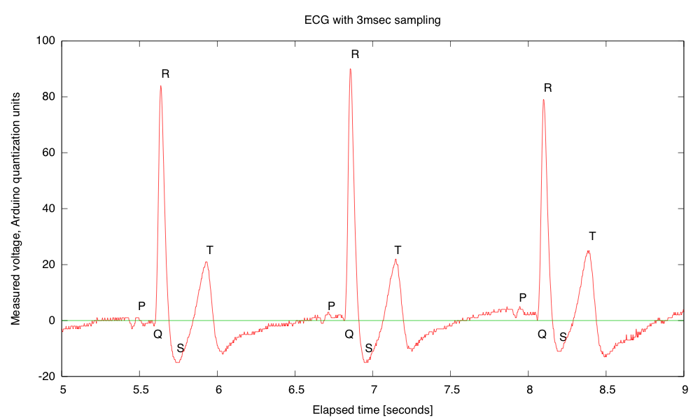
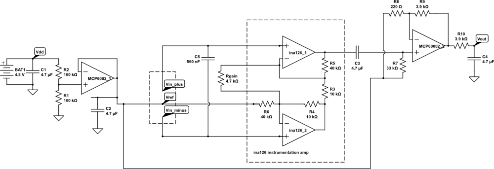
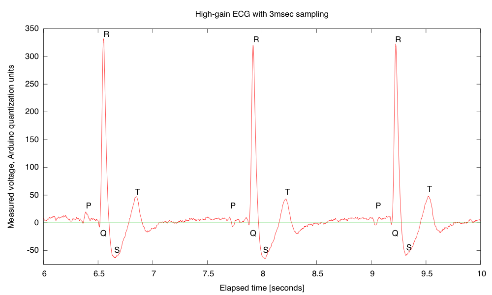
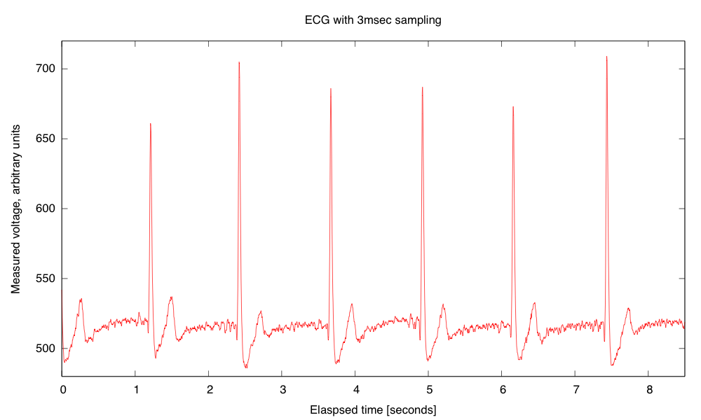
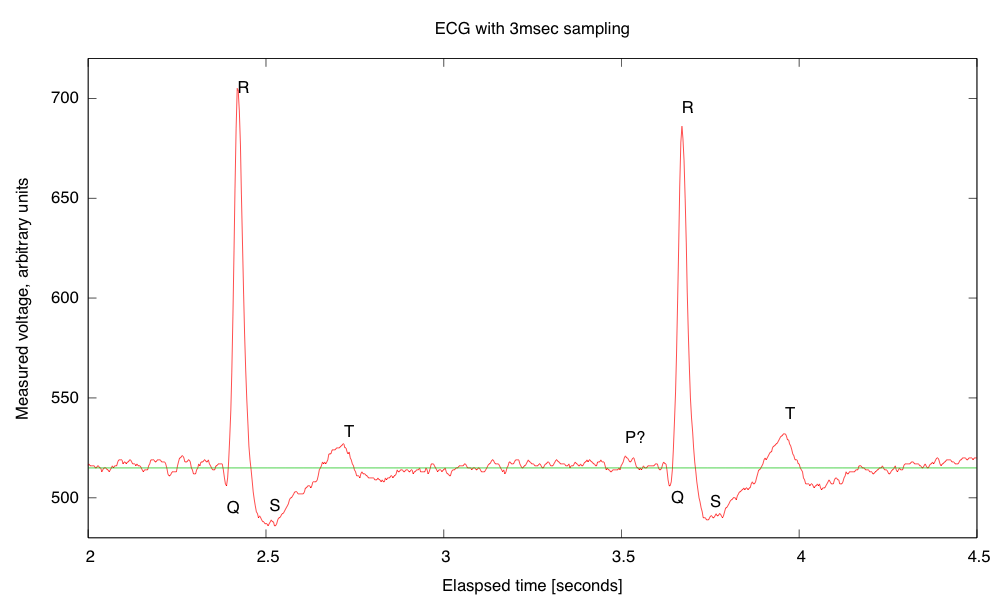
The electrocardiogram will be the final project for the course, and I think it will take two full lab sessions. The first lab session would consist of soldering up the instrumentation amp protoboard, checking for opens and shorts, and designing and characterizing a differential amplifier with an adjustable gain of about 100–1000 (including AC coupling to eliminate problems with DC offset saturating later stages).  The amplifier should have a bandwidth of about 0.01Hz–150Hz.

The second one would be and making a twisted-wire harness with alligator clips to attach to the EKG electrodes, connecting the amplifier to the electrodes, debugging the student-designed EKG amplifiers, and adjusting the gain.  I suspect that a few students will get a design that works in the first week, but that a lot of students will be doing a lot of unsoldering and resoldering as they find bugs in their design, hence the need for 2 weeks in the lab.

Student check out will require that they be able to blink an LED in time with their heart beat, display the EKG waveform on the oscilloscope, and record a minute of EKG signal at 200 samples/second using the Arduino, all without adjusting their board between demos.

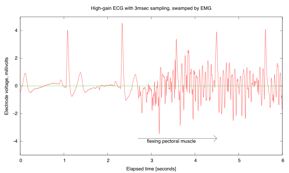
EE concepts: biopotentials, instrumentation amplifier, common-mode signal, differential signal, twisted pair wiring, grounding to avoid common-mode signal saturating an instrumentation amplifier, Ac coupling, simple bandpass filtering.

Lab skills: soldering.

Summary

I have a pretty clear idea how I think the lab part of the course should start and how it should end, but there are a couple of weeks just before the end that are still a bit vague.  Perhaps as Steve starts aligning the EE topics with the labs he can identify some topics that need a lab exercise to clarify them.  Maybe some of my blog readers (those who haven’t deserted me during this long process of designing a course) can make some more suggestions—even repeating some old suggestions would not be a bad idea now, as I need a creative kick.

Before doing the EKG lab, we should definitely discuss safety concerns,  including things like the following chart (information from http://electronicstechnician.tpub.com/14086/css/14086_34.htm):

The very small voltages we work with (5–10 V DC) means that we rarely need to be concerned about safety issues in the lab. Most of the resistance of the body comes from the skin, and varies enormously according to how sweaty the skin is. Cleaning dead skin cells off (as is done with most preps for EKG electrodes) reduces the resistance of the skin quite a bit. DC is somewhat safer than AC, because skin is less conducting than the rest of the body, and so acts as a capacitor in parallel with a resistor. Puncturing or scraping the skin reduces resistance considerably.

It would probably be useful to have students measure the resistance between two Ag/AgCl electrodes and compute the currents that would flow at different voltages. When I tried this on two chest electrodes (just after showering, so clean, damp skin) I measured around 50kΩ. Pressing the electrodes more firmly against the skin dropped the resistance to 25 kΩ, and it gradually crept back up.

I keep thinking that the 3-wire design for EKGs is overkill. The 3rd wire seems to be just provided to bias the body to be between the power rails of the instrumentation amplifier. It should be sufficient to bias one of the electrodes with a large resistor to the reference voltage directly, rather than through the body.

I tried this.  First I hooked up the 3-wire system of the 2-stage EKG amplifier (though there was a mistake on that post, as the Rgain resistor was really 4.7kΩ, not 820Ω).  This was to make sure that I was getting good contacts and a clean signal. I then disconnected the bias lead and tried to bias the opposite end of the wires.  This did not work at all.  Disconnecting the bias wire resulted in a large signal with a period of 16.7ms (60Hz, though with a complex waveform).  Adding resistors between Vplus and Vref, Vminus and Vref, or both, just made this noise worse.  I then tried taking my body out of the loop, connecting a 25 kΩ resistor between the clip leads.  Without the biasing resistors I saw the same complex 60Hz signal.  It seems to come from capacitive coupling to the leads, as moving my hand closer or further from the leads changes the magnitude of the signal, and grounding myself eliminates it.  Putting 24kΩ resistors between Vplus and Vref and between Vminus and Vref reduced the noise, but did not eliminate it.  Touching either Vplus or Vminus was enough to produce huge noise again.

I tried another experiment, where I attached the ground electrode not to Vref directly, but through a 0.56 μF capacitor.  This worked fine, even though there was no DC bias connection for the instrumentation amp inputs!  It stopped working if I then touched either the +5V or 0V power rail—the DC bias is important, but my body was working as a pretty good capacitor, holding the DC bias for quite a while.  It is clear that the AC path to ground is crucial also.

I found that I could clean up the EKG signal by putting a 0.56 μF capacitor between Vplus and Vminus—enough that the P part of the EKG was visible.

Clean EMG with P,Q,R,S,T parts of signal all clearly visible. The remaining noise seems to be mainly quantization noise in the Arduino analog-to-digital converter, which could be reduced by increasing the amplifier gain.

Since the remaining noise seemed to be all quantization noise, I upped the amplifier gain.  Trying to raise the gain on the first stage did not work, so I raised the gain on the second stage.

Higher gain EKG circuit, with capacitor on the inputs.  The first-stage gain should be 22.02, and the second stage  18.73, for a total gain of 412.4.

The higher gain amplifier did produce good traces, with less evidence of quantization noise:

The “Arduino units” are 4.967 V/ 1024 = 4.851 mV at the output of the EKG, or 11.76µV at the electrodes. The R peaks are about 3.9mV and the S dips about -0.7mV.  The first R-R interval is 1.368 seconds for a pulse rate of 43.86 bpm.

One thing that is important—the EKG readings are resting EKGs.  If I flex the left pectoral muscle, I can swamp out the EKG signal.

Every EKG is also an EMG (electromyograph), and flexing muscles between the electrodes (here the left pectoral muscle) can swamp out the EKG signal. I computed the electrode voltage from the recorded signal, the measured Arduino A-to-D reference voltage, and the gain of the EKG amplifier. The zero-reference is determined by recording the Vref signal as well as the EKG output signal. The quantization noise from the A-to-D converter is about 3μV (less than 1 pixel in this picture).

My son and I spent some time today debugging his data logger.  I also convinced him to add some documentation, though not nearly as much as I think is needed.  This version is just a text command interface, with no GUI—the PyGUI interface he was building seemed to slow things down a lot, and is not yet ready for use.

The data logger works fine as long as the sampling interval is at least 3msec.  With 2msec sampling, I think that serial communications (over a 115200 baud USB serial connection) is getting overwhelmed.  The Arduino seems to be capable of sending out data ok at 2msec/sample, though 1msec/sample causes it to miss some timer interrupts.

If the Python program can’t empty the serial port fast enough, I think that there operating system problems. My MacBook Pro sometimes gets wedged with long runs at higher sampling rates—I’ve had to reboot it a couple of times today. If the problem is with the MacBook Pro, it may be possible to run with slightly shorter sampling intervals on faster hosts, before hitting the limits of the Arduino.

I did manage to get a nice recording for about 8.5 seconds at 3msec sampling:

Recording of EKG trace on the Arduino. The value 512 represents the midpoint of the Arduino voltage scale. The EKG circuit and Arduino used separate power supplies, so the reference voltage is about 2.506V, while AREF on the Arduino was 4.96V, so the reference voltage should be about 517.  In a separate recording of the EKG signal and Vref, I found Vref to be 515±1.  The arbitrary units are about 4.844mV at the input to Arduino.  If my gain of my EKG is set to 591 as I expect from the resistor values, the arbitrary units should correspond to 8.2µV at the electrodes, and the biggest peak is about +1.6mV and the deepest drop is about -0.24mV.

I think that the signals were clearer today, because I was using a ground electrode on my chest, rather than on my elbow, reducing the common-mode noise a little. The 3msec resolution allows zooming in to get a pretty clear view of the structure of the pulses:

Detail of a couple of pulses showing the QRS complex and the T pulse. I’m not sure whether or not a P pulse is visible—if so it is almost buried in the noise. I’ve added a line where I believe that the reference voltage is, though it was not recorded on this run. The R-R interval here is about 1251±2msec for a pulse of 0.80 Hz or 48.0 bpm, which is about my usual resting pulse.

Although it took my son and me a little debugging to get everything working today, overall I’m quite pleased with the data logger code he wrote. He still has more documentation to add (both in-code and external), and there are some more features that could be added, but it is basically usable as is.

Incidentally, I found out today from Cardiology Explained by E.A. Ashley and J. Niebauer, that

ECG terminology has two meanings for the word “lead”:

• the cable used to connect an electrode to the ECG recorder
• the electrical view of the heart obtained from any one combination of electrodes

So it is not surprising that I was confused by the usage—I was only familiar with the first usage, which corresponds to normal engineering terminology.

In Learning to Use I2C and Magnetometer not fried, I talked about interfacing the MAG3110 magnetometer and MQA8452Q accelerometer to an Arduino.  For both, I’m using breakout boards from Sparkfun Electronics.

I  checked today that there are no problems when I connect both devices to the same I²C bus.

The first test was very simple: I put both the breakout boards into a breadboard and wired them together, then tried running each of the programs I’d written for the chips separately. Result: no problems—worked first time.

I then tried merging the programs (cleaning up any naming conflicts) so that both could be run from the same code.  After a few typo fixes, this also worked fine

I think I’m now ready to hand over the software to the students to use for their robot.

I still need to put the i2c.h, i2c.cpp, and accel_magnet code in some public place for others to use (perhaps on github? maybe on my web pages at work?) [UPDATE 2012-jan-31: I have put the libraries and the sample code for the accelerometer and magnetometer at http://users.soe.ucsc.edu/~karplus/Arduino/]

One thing that is still missing is doing tilt correction for the compass heading.  Since the ROV is not expected to remain level (the accelerometer is intended to be used in a feedback loop to adjust the pitch, with anything from -90° to +90° being reasonable), getting a good compass heading requires rotating the magnetometer readings into the horizontal plane.  Only one of the students in the robotics club has had trigonometry or matrix math, so I’ll have to work with him to get him to figure out how to do the tilt correction. It may be simplest conceptually  to compute pitch and roll angles first, then rotate twice, rather than trying to do the whole tilt correction in one step (especially since the Arduino does not have matrix libraries).

Related articles

• Learning to use I2C (gasstationwithoutpumps.wordpress.com)
• Soldering problems (gasstationwithoutpumps.wordpress.com)
• Magnetometer was not fried (gasstationwithoutpumps.wordpress.com)
• Tilt compensation when reading a digital compass (hackaday.com)

For the Santa Cruz Robotics Club, I’ve bought three sensors for their underwater ROV: a magnetometer, an accelerometer, and a pressure sensor.

Originally, we were going to an ADXL335 accelerometer (with a breakout board by Adafruit Industries) and an MPXHZ6250A pressure sensor (no magnetometer), for which I designed a small PC board, but once the specs for this year’s mission came out, we saw that they wanted us to determine compass headings for a “sunken ship”, so it seemed a natural thing to add a magnetometer to the hardware.  After looking at what was available, I chose the MAG3110 breakout board from Sparkfun, because it provided a triple-axis magnetometer for only $15.

The MAG3110 is an I²C interface, which means we need only 2 wires to hook it up (and the wires can be shared with other I²C devices).  If we are going to all the trouble of figuring out an I²C interface, I figured we might as well use it for the accelerometer as well, so I got a MMA8452Q breakout board from Sparkfun also.

I decided to do a simple test program for the I²C parts before handing them over to the robotics club, so that they could be sure they had working parts.  It was a good thing I did, because I spent more than an entire day trying to get the parts to work.  I finally gave up on the “Wire” library from the Arduino website, and tried using the i2c.h file from Sparkfun (example code linked to from the accelerometer web page).  I got that working and rewrote the library as a proper .h and .cpp file, so that it could be installed as a normal Arduino library, adding some of the utility calls that had been buried in the MMA8452 demo code.

The MMA8452Q code was working fine, so I tried using the same i2c library for the MAG3110 magnetometer.

I had gotten MAG3110 working with the Wire library, but running at 5v (I’d not noticed that it was a 3.3v part—rather, I thought I’d checked that it was a 5v part, but I was wrong).  I’d left it powered at 5v all night, and I think I burned it out, as it was quite warm in the morning.  Today, I can read and write the registers of the MAG3110, but the xyz values are not coming out reasonable at all—I frequently get the same values (like 0xF9F9)and 0x1DF9), independent of the orientation. If I read all the registers, a lot of them come out as 0xF9 or 0x1D.  Even the WHO_AM_I register (which should be 0xC4) often comes out 0x1D.  I seem to get intermittent correct values for registers, but mostly bogus values.

I’ll feel stupid if I order another part and it turns out to be a software bug, but I’m pretty sure the chip is fried.  But I guess it is time to do another Sparkfun order. (I owe them some business, after calling them for the replacement photointerrupter.)

Incidentally, I tried finding a usable pressure sensor with an I²C interface, but it doesn’t look like anyone is making them except for barometric pressure ranges for dry gases.  I suppose Freescale will eventually come out with a full range of I²C pressure sensors, but my guess is that will be a long time coming, as the automotive and industrial applications have a pretty long product design cycle (unlike consumer electronics, which is driving the barometric pressure sensors).

In today’s lab we derived the formula for the period of a simple pendulum (assuming the small-angle approximation), , then measured both circular and simple pendulums.  For the circular pendulum we measured the radius of the cone on the first orbit and the last orbit, the length of the string (the slant height of the cone), and approximated the period by timing 10 or 20 periods and dividing.  For the simple pendulum, we used the photogate setup described in More on pendulums, to get very precise and repeatable measurements of the period.  The hardest part for us was measuring the length of the pendulums, since the center of mass for the bob was not obvious and the exact position of the pivot was not obvious—these uncertainties probably resulted in length measurements being ±5mm, making a large contribution to inaccuracy.

Here is a table of the measurements (and calculated g) we made for the circular pendulum:

The range of estimates for g is larger than I would like.  I think that the decay of the oscillation of the pendulum makes quite a difference.  The average of all the estimates of g is 967 gm/sec^2, which is rather low.

And for the simple pendulum:

The pendulum ticked reliably for quite a while, and the periods were remarkably consistent.  The estimates of g from the simple pendulum are good to about 0.5%, which is the limitation of accuracy on our pendulum length measurements and close to the limit of the accuracy of the small-angle approximation.  The average of the 5 measurements looks good to about 0.2%, which seems pretty good to me, since we certainly weren’t measuring the lengths that accurately.

I looked up the gravitational field in Santa Cruz on Wolfram Alpha’s gravitational fields widget:

total field | 9.7995 m/s^2  (meters per second squared)
angular deviation from local vertical | 0.00322°  (degrees)
down component | 9.79945 m/s^2  (meters per second squared)
west component | 3.4×10^-4 m/s^2  (meters per second squared)
south component | 0.0316 m/s^2  (meters per second squared)
(based on EGM2008 12th order model; 11 meters above sea level)

While the lab was running, one of the students wrote a Python script (using numpy for mean and standard deviation) to read the data and compute the numbers in the table.  We could have talked directly to the Arduino, but it was simpler to cut the numbers from the Arduino serial monitor and paste them into a file for the script to read. That allowed us to keep the Arduino running throughout, and just cut and paste the good numbers, discarding the junk from starting or stopping the pendulum.

I’m quite pleased with the photogate setup, which was very simple to build and worked reliably during the experiment. Crudely wrapping tape around the string made a lumpy opaque object, whose rotation probably contributed to the standard deviation of the  period—having a smoother cylinder for the optical blocker would probably make the period measurement much more consistent.  But that would not improve the mean estimates much since errors in adjacent period measurements cancel.  I believe that our mean periods are much more accurate than the standard deviations suggests, with errors less than 1 per thousand.

I had to make one change in the Arduino code during the lab to accommodate all the different pendulum lengths—I had a dead time before recognizing the next pulse, to prevent getting 2 pulses per period as the string passed through the beam twice.  I started with a dead time of 1 second, which as a bit too long for the smallest pendulum.  Reducing the dead time to 500 msec for that pendulum made it count reliably.  Note that for the 2nd and 3rd pendulum, we measured for about 3 minutes without a bad time measurement, and could have gone longer if we had had the patience.

In Newton’s measurement of g, I described a failed experiment to measure g with a motorized circular pendulum. Further experimentation on my own lead me to adopt for this week’s lab the standard approach using an unpowered circular pendulum.  The cone formed by the string can be described as having height , base radius , and hypotenuse , the length of the string.  If the circular pendulum has period , then (derived in the Newton post).  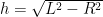If we make the string long and push the pendulum with the right speed to get a nearly circular (rather than elliptical) motion, then is nearly constant for many orbits, and we can estimate the period with just a stopwatch by counting 20 or 30 periods.  Using a large enough mass means that neglecting air resistance is now reasonable (which it was not for the tiny mass I started with).

Thanks to John Burk for suggesting that I forget about the motor—that seems to be the best approach, even though I then can’t use the photogate to time the period.  I’m hopeful that we can measure the height and the period accurately enough to get within about 2% of the right value for .

This week in addition to doing the circular pendulum right, I wanted to do simple pendulums.  I’ve assigned problem 4.P.89 in Matter and Interactions, which seems to be the only place in the book that simple pendulums are done.  It is a computational problem, since there isn’t an analytic solution (though the small-angle approximation works pretty well up to about 45°).  I hope the students have done that by tomorrow!

I wanted to measure the period of the pendulum directly (not averaging over many periods), to demonstrate that the amplitude does not matter much.  Unfortunately, I’ve not yet built a sensor that works for this. I tried using the photogate, but I could not hit the 1 cm gap consistently, even with a shorter pendulum.

I also tried using a magnetic sensor (using the circuit I used for the speed-of-sound lab) with a magnet for the pendulum weight, but that triggered at random times as the magnet came close.  Even 20cm away the field was enough to trigger the detector, and I got almost random timings.  A magnetometer was no better than the coil and comparator, as the magnetic field varied chaotically (from movements of the magnet other than the simple pendulum swing, such as twirling on the string).  The magnetometer was usable as a compass, though, which is good, because I originally bought it for the robotics club to use as a compass.  There are some tricky points to using it as a compass, which I’ll talk about in a different post.

I then tried marking the top of the string with a bit of electrical tape and using the photogate there.  That was the most successful so far—if I hold the photogate steady enough, I can get readings repeatable to ±20msec, which is much better than I can do with any other approach I’ve tried.  For one pendulum hanging from the edge of my desk, I either got  two pulses at about 1.11 and 0.45 seconds or one pulse every 1.56 seconds, depending on whether the marker on the string passes all the way through the beam or blocks it continuously at the end of the swing. The random variation I get is probably because of holding the sensor by hand (to align with the string).

If I had a more rigid way to mount the sensor, I should be able get more consistent readings, so my main engineering task was to get a rigid pivot point on the ceiling beam (without making any holes) and mount the photogate in a rigid, but adjustable, way.  Of my two standard mechanical engineering techniques, duct tape and Lego, I chose Lego:

A view of the photogate mounted on the Lego beam next to the pendulum string.

Closeup of the photogate, showing the breakout board and sensor wedged between a plate and a beam, with a 2-plate spacer.

Having come up with a nice way to grip the photogate and still be able to swing a pendulum string into the gap, I connected the beam holding the photogate to the same right-angle platform that we had used last week for the motorized pendulum. This left a little gap that I could rest the Arduino board in, so that there was no tension on the wires to the photogate.

I was a bit worried that I might have to put my laptop on top of a ladder, since the USB cord is not very long, but I have a spare pair of USB-to-Cat5 converters (one set is for the robotics project), so I was able to make an extension cord out of a flexible Cat-5 Ethernet cable, giving me enough length to put my laptop safely on the desk.

The same Lego that holds the photogate can also support the Arduino, so I don't need to hold anything in my hands.

I had two other ideas I haven’t tried: using one of the ultrasonic range finders to track the pendulum motion and using a video camera to time the motion.  These require interpolation of position data to estimate the period, so I’d rather avoid them for now. The top-of-string photogate will work (I think) for the simple pendulum, and the circular pendulum can be timed with a stopwatch averaged over many periods.  (I could even use the photogate timer as a stopwatch, though the resolution of the stop watch on my Casio wristwatch is 0.01 seconds, and human reflexes make anything less than 0.1 second pretty much noise.)

The speed-of-sound lab we did on 30 Dec 2011 went pretty well after all.

Coil (about 0.5H) with refrigerator magnet on top. Magnet is stuck to the core of the coil just by its own magnetism.

I used a setup inspired by the one in the Chapter 4 Lecture 3 video at http://courses.ncsu.edu/py581/common/podcasts/.  That is, a long metal bar tapped with a metal striker at one end.  A clock is started when the tap is made (a simple electrical connection), and stopped when the wave is detected at the other end.  As mentioned in my earlier post More on the slinky and the speed of sound, I used an electromagnet and a small refrigerator magnet to detect the sound wave.  The coil has a  68.3 Ω resistance and a laminated iron or steel core, and I estimated the inductance at about 0.5 Henry (the estimate  may easily be off by a factor of 2—I should measure it better some day when it matters). When I rested a piece of aluminum bar stock on the magnet and tapped the other end, I got a signal of about 0.3 v, which I could see clearly on my oscilloscope.  (Note: the analog view of the signal was not done in the lab with the students, because we were pressed for time and moving the analog oscilloscope out to the room worked in and setting it up would have taken too long.)

The signal is not large enough to be measured by a digital input on the Arduino that we used for timing, and the Arduino analog-to-digital converter (accessed with analogRead()) is a very slow one, that would limit our time resolution to about 100 µsec, rather than 4 µsec as we can get with the “micros()” function call. I happened to have an LM311 comparator chip from about 30 years ago, so I made a comparator circuit to convert the analog signal to a clean digital signal.

Comparator circuit used to convert the small electrical signal induced in the coil to digital levels for input to the Arduino. The pair of 15kΩ resistors serve as a voltage divider to set the bias voltage for the inputs to about 2.5 volts, in the middle of the range. The output pull-up resistor provides a load for the comparator. The two capacitors filter out high frequency signals picked up by the coil—they were not part of the circuit provided in the LM311 datasheet, but turned out to be essential.

I did have to modify the circuit a little from the one for a magnetic pickup given in the data sheet, as the output remained high with that circuit.  Adding small capacitors to the input and output seemed to fix things.  I arbitrarily used 47000pF capacitors, because I happened to have several of them, but I also experimented with some other sizes (560 000 pF and 1000pF) which did not work.  One effect of the capacitor on the input is to make a resonant circuit that rings with a period of about 800 µsec (eyeballed from the oscilloscope trace), which would make the inductance of the coil about 0.34H.  This ringing has a couple of consequences: 1) if the magnet is the wrong way around, the polarity of the impulse is reversed and the comparator will detect the impulse half a cycle later, adding about 400 µsec to the reading, and 2) the signal ramps up slowly in response to an impulse, and the delay in the comparator circuit is dependent on the magnitude of the input signal.  This will add noise to the timing measurements.

Because the magnet we used had residues of paper and glue on one side, it was easy to check that it was oriented correctly.  For one set of measurements, the coil and magnet had to be moved, and the magnet may have been upside down for that set of measurements, resulting in a different offset for those measurements.

To keep the noise from differences in amplitude to a minimum, we took several measurements (generally 10 or 20) of each time, discarding obviously bogus numbers (like 8 µsec when the comparator had already detected something before the strike, or > 10 msec, when an impulse had been missed).

On the Arduino, the following program was used measure times.  Pin 2 of the Arduino was connected with a long wire to a metal striker, with the object being struck connected to Arduino’s GND with another wire.  Contact between the two metal objects pulled pin 2 down (overpowering the 20kΩ pull-up in the Arduino), recording the time in start_1. As soon as the comparator detects the sound, pin 3 is pulled down, and the time is recorded on stop_1.  The resolution of the timer is about 4 µsec, but the repeatability of the times varied more, depending in part on how consistently the strikes were made (one of us appeared to have much more consistent technique than the others, and the times from his strikes had lower spread—we did not record who did the strikes on our data log, and so we can’t quantify this observation).

void setup()
{
  //  put a 20k pullup resistor on pin 3 (sound detector)
  pinMode(3,INPUT);
  digitalWrite(3, HIGH);
  //  put a 20k pullup resistor on pin 2 (striker)
  pinMode(2,INPUT);
  digitalWrite(2, HIGH);

  Serial.begin(115200);
}

void loop()
{
  Serial.println("Ready");

  // wait for pin 2 to go low (contact with striker)
  while (digitalRead(2)>0) {}
  long start_1=micros();

  // wait for pin 3 to go low (sound detected)
  while (digitalRead(3)>0){}
  long stop_1=micros();
  long diff = stop_1-start_1;
  if (diff > 10000)
  {   Serial.print(F("rejecting large delay: "));
  }
  Serial.print(diff);
  Serial.println(F(" microseconds"));
  delay(200);  // wait 200 msec

  // wait some more if the striker still in contact
  while (digitalRead(2)==0) {}

}

The vertical rod is the one being measured. The sensor is on the floor and the rod is struck at the top end. The breadboard has the comparator circuit connected to the Arduino, which in turn is connected to a laptop (not in the photo).

The setup for most measurements was simple: the coil was put on the floor with the magnet resting on top. A rod was held vertically on top of the magnet and struck at the far end with another rod. Initially, we used a small screwdriver as the striker, but this turned out to be hard to hold, and so we switched to using a foot-long piece of ¼” steel rod, which was also used for some of the timing tests.

Because the delay in the comparator is unknown, but likely to be substantial compared to the time of flight, we tried to measure the same material at different lengths, and do a straight-line fit of the data to estimate the offset. By doing many measurements at each length, we could average out a lot of the noise. We could also see how well the data fitted a model that assumed that the time delay for the sound arriving would be proportional to length—that is, does the speed-of-sound model make sense for this data?

The simplest set of data was for 3 rods ¼” in diameter, made of hot-rolled weldable steel (that’s all the information about the material that the hardware store had on the tag). I’ve put the data in a page on the blog: Steel rod speed of sound lab data.

We also measured one aluminum bar (Aluminum bar speed of sound lab data), one long copper tube (Copper tube speed of sound lab data), and two wood dowels (Wood speed of sound lab data).  Because wood is not conductive, we added a washer on the striking end of the dowel, to provide a conductive contact. The copper tube was about 3m (10′) long and very soft, so we laid it on the floor and duct-taped the sensor to one end.

Perhaps the most interesting data set comes from an aluminum ladder (Aluminum ladder speed of sound lab data).  We removed one foot from the ladder and duct-taped and bungey-corded the sensor to the bottom of the ladder.  We then struck the ladder inside the hollow rungs, providing a nicely spaced series of different ten different lengths.  Because of the difficulty in getting the duct tape to stick to the ladder, the magnet fell off and was replaced a few times in setting up the sensor.  The final orientation was not checked, but I believe that it was backwards, so that the delays of the sensor were substantially larger for the ladder than for the other measurements.  Luckily, there are enough different lengths that we can get a very good linear fit even with a large offset.

I did a fit for the steel-rod data using the following gnuplot script:

unset key

set title "Time of flight for compression wave in 1/4\" hot-rolled steel rod"
set xlabel "length (meters)"
set ylabel "time (seconds)"

set xrange [0:*]
set yrange [0:*]

fit a*x+c 'steel-rod.txt' using (0.01*$1):(1e-6*$2) via a,c

print "velocity=", 1/a, "m/s"

plot a*x+c, 'steel-rod.txt' using (0.01*($1+2*rand(0))):(1e-6*$2)

which produced an estimate of 5292 m/s for the speed of sound in the steel rod. I was noticing on the web that the speed of sound in thin rods may be a bit different from the speed of a planar wave in bulk steel, so I’m not sure what the “right” value is for this measurement, but it sure seems reasonably close to reported values around 5000–6000 m/s.  I also get from the same fit an estimate of the delay in the sensor and comparator of 33.7 µsec, which I can use for the aluminum bar and copper tube data. How does the fit look?  See for yourself:

The linear model seems like a pretty good fit for the data on the steel rod, but the scatter on the data is a little high. Note: small random jitter was added to the x values, in order to spread the points out.

If I remove outliers (the two largest and two smallest measurements from each length), I get a tighter fit (naturally), but one with is also likely to be more accurate, as outliers have a large influence in linear regression:

After eliminating the outliers, the estimated speed of sound is 5267 m/s and the sensor delay is 31 µsec.

Using a similar script, but with a fixed 31 µsec offset, for the aluminum bar data and the copper tube data (again eliminating the two largest and two smallest measurements), we get 4412 m/sec for the aluminum bar and 3857 m/s for the copper tube. (Of course, we don’t have anywhere near 4 significant figures, so I should probably round these to 4400 m/s for aluminum and 3900 m/s for copper.)

The ladder data used essentially the same script as the steel-rod, but even after censoring the data had a pretty wide spread:

The ladder data, after removing the two largest and two smallest times at each data point, got an estimated speed of sound in aluminum of 3955 m/s. The offset was 256.6 µsec, confirming that the magnet had been reversed. (It also implies that one period of the ringing is about 450 µsec, which is shorter than the period I thought I saw on the oscilloscope.)

If I fit the data from the wood dowel using the 31 µsec offset, the line does not fit the data at all well. If I fit with a 2-parameter model, I get an offset of 162.6 µsec (between the ones for the steel rod data and the ladder data), and a velocity of 6150 m/s, which is unusually high for wood. It is a very light wood, so perhaps the number is reasonable, but I’d be more comfortable if we had had more different lengths to test. The difference in the delay introduced by the sensor suggests to me that I should have used multiple lengths for each of the materials, despite the inconvenience (I only had one piece of aluminum bar and did not want to cut it—similarly, I did not want to cut the copper tube.)

Comparing our speeds with typical speeds from engineeringtoolbox.com:

The best match is for the copper, with our aluminum alloys having a much lower speed of sound than typical for pure aluminum (does our alloy have higher mass? lower stiffness?), and our wood dowel having a much higher speed of sound than typical for wood. The steel rod was a little low, but within the range of reported speeds of sound in steel.

This report took me several hours to write, in part because producing the graphics took a while, and in part because I fussed around a lot with seeing if removing outliers from the data helped get better results.  My son produced a substantially similar lab report, with graphs but no pictures or schematic of the comparator, in 2–3 hours.  He did not play with removing outliers.  He also correctly reported the velocities with only 2 significant figures (in cm/µsec).