Adjust the phase current, crank up the microstepping, and forget about it — that’s what most people want out of a stepper motor driver IC. Although they power most of our CNC machines and 3D printers, as monolithic solutions to “make it spin”, we don’t often pay much attention to them.

In this article, I’ll be looking at the Trinamic TMC2130 stepper motor driver, one that comes with more bells and whistles than you might ever need. On the one hand, this driver can be configured through its SPI interface to suit virtually any application that employs a stepper motor. On the other hand, you can also write directly to the coil current registers and expand the scope of applicability far beyond motors.

Last month, we took a closer look at microstepping on common stepper driver ICs, but left out the ones that we actually want to use: the smart ones. Trinamic provides some of the smartest stepper motor drivers on the market, and since the German hacker store Watterott released their SilentStepStick breakout boards for the TMC2100 and TMC2130, they are also setting a new standard for DIY 3D printers, mills and pick-and-place robots. I recently acquired a set of both of them for my Prusa i3 3D printer, and the TMC2130 with its SPI configuration interface really caught my attention.

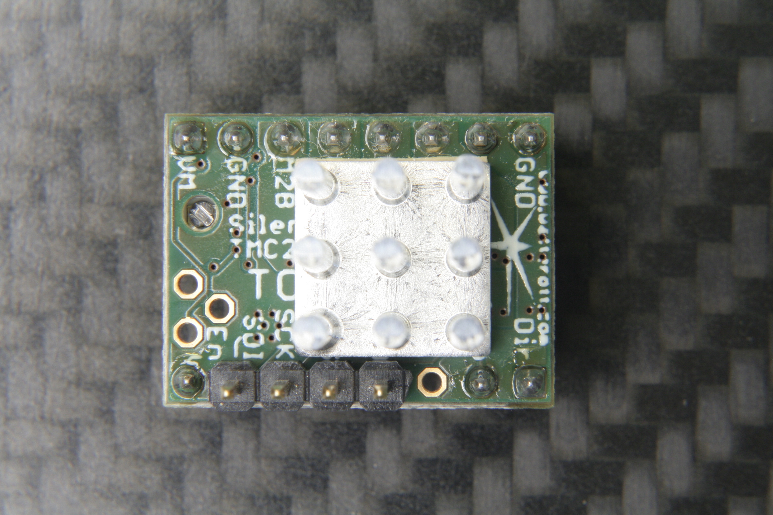
The TMC2130 SilentStepStick should not be confused with the — far more popular — TMC2100 variant. As the name suggests, it comes as a StepStick-compatible breakout board, and just like it’s famous sibling, features a Trinamic IC on the bottom side of the little PCB. Several vias and copper spills conduct heat away from the IC’s center pad, allowing a heatsink on the top side to effectively cool the driver.

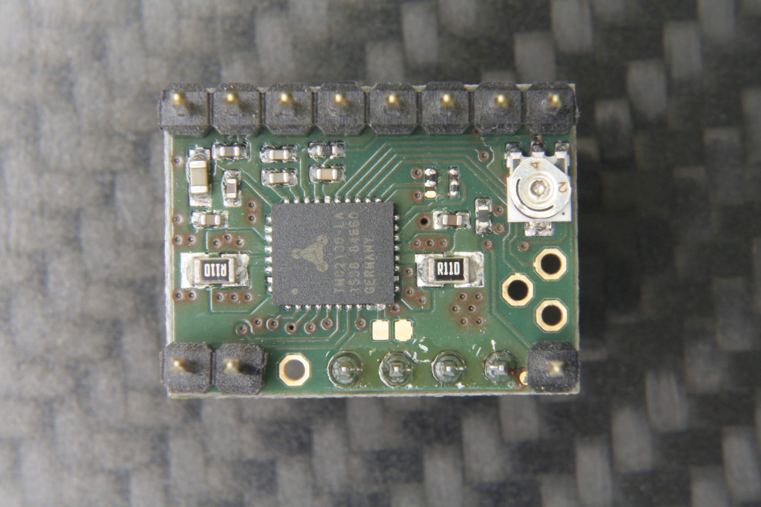
However, unlike the TMC2100, this one won’t let your motors spin right away. You’ve got two options: Hard-wire it in stand-alone mode, which practically turns it into a TMC2100, or hook up to its SPI-interface and dial in if you want your stepper motor shaken or stirred. In fact, plentiful configuration registers make the TMC2130 an extremely hackable chip, so I’m not even thinking about bridging that solder jumper on the SilentStepStick’s bottom side that activates the stand-alone mode.

First Steps

As said, before the driver does anything, it wants to be configured, and it’s worth mentioning that all configuration registers are naturally volatile, so if I want to use them in my 3D printer, I need to configure them as part of the printers startup routine.

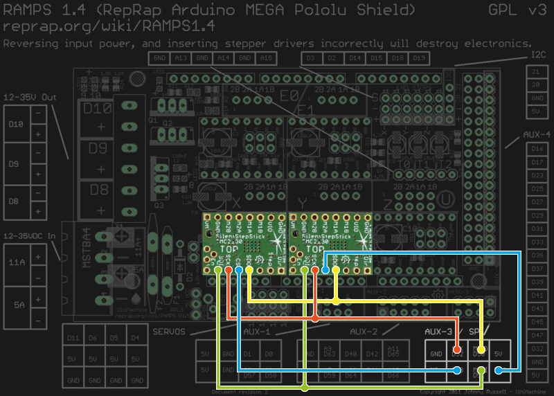
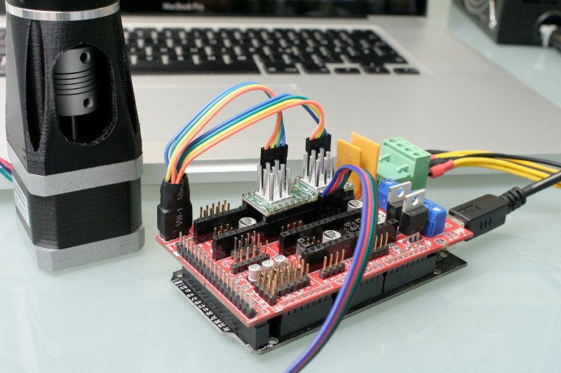
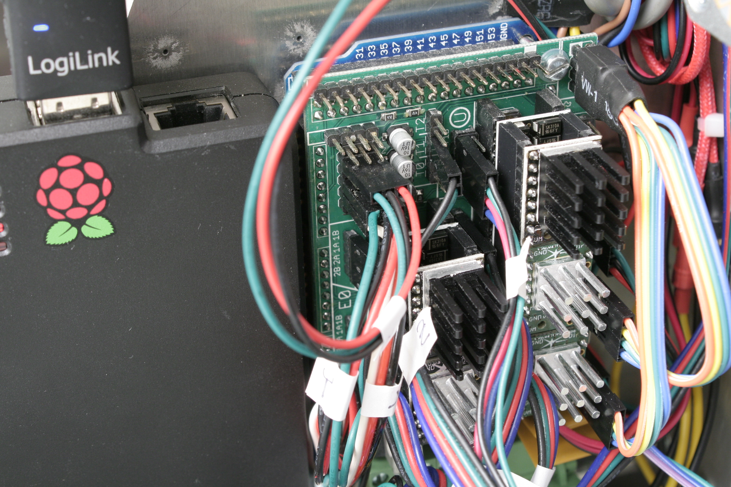
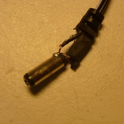
The RAMPS 1.4 on my 3D printer breaks out the hardware SPI interface of the underlying Arduino through its AUX3 pin header, along with two additional digital pins (D53 and D49), which I used for the cable select signals. After crimping a cable to connect two TMC2130’s to the AUX3 header, I could start digging into the software part.

Watterott provides an example sketch, which writes a basic configuration to the driver’s registers and spins an attached stepper motor. Great stuff, but the datasheet describes 23 configuration registers waiting to be finely tuned, and 8 more to read diagnosis and status data from. So, I wrote a little Arduino library that would make the numerous configuration parameters available in a more practical way. From there, I could just include my library into the Marlin-RC7 3D printer firmware I’m using. Luckily, the current Marlin release candidate already features support for TMC26X drivers, so I could reuse some of its code to put together a Marlin fork that includes 59 of the TMC2130’s parameters in its define-based configuration files. And then, I could take the little buddies out for a spin.

Taking Them For A Spin

With the hardware set up and the software working as supposed, I ran a few sanity tests: toggling parameters on and off and checking how the driver’s behavior changes during printing. Since the TMC2130 let’s you tune almost everything it’s doing, that’s a good first step that helps to eliminate some variables and picking others that are worth a deeper look. Most of the settings can be changed on the fly and mid-print, however, not all parameters can actually be safely changed while the motors are running.

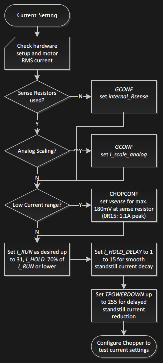
To actually tune the drivers for a certain application, Trinamic provides a quick start guide in the datasheet, as well as detailed information on each parameter, and on how they interact. Basically, the first step is adjusting the RMS coil current by using the onboard potentiometer on the SilentStepSticks. Then, we need to chose the analog input pin as a current scaling reference to actually make use of the potentiometer. The mentioned library lets me do this through a simple method:

myStepper.set_I_scale_analog(1); // 0: internal, 1: AIN

The running and holding current are the first real parameter that should be tuned, with the running current typically at the desired maximum current, and the holding current at 70% of this value. The delay between a stillstand and the transition from running current to holding current can be adjusted between 0 and 4 seconds, and for now, I set it to 4 seconds, practically disabling the current reduction while the 3D printer is running. The three values share one write-only register, so the corresponding method call looks like this:

myStepper.set_IHOLD_IRUN(22,31,5); // [0-31],[0-31],[0-5]

and sets the running current to 100% (≙ 31), the holding current to about 70% of this value (≙ 22), and the delay between the two to 4 seconds (≙ 5).

I want torque, so I can leave stealthChop disabled. The datasheet suggests some starting values for configuring the chopper’s off time and the comparator’s blank time settings, but since it’s a key tradeoff between switching noise and torque, it makes sense to iterate through other values as well. The library methods for the two values look like this:

myStepper.set_tbl(1); // [0-3]
myStepper.set_toff(8); // [0-15]

And finally, I need to pick a microstepping resolution and choose if I want to make use of the 256 microstep interpolation feature, covered later in this article:

myStepper.set_mres(32); // {1,2,4,8,16,32,64,128,256}
myStepper.set_intpol(1); // 0: off, 1: interpolate

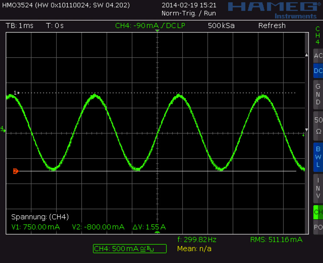
I have yet to walk through the entire tuning procedure, which includes monitoring the coil current on the scope and eliminating distortions in the zero crossing, but I’m getting a clue of the driver’s potential.

Juice

It’s maximum continuous RMS current of about 1.2 A per coil (at least in the QFN package on the SilentStepSticks) lets it look like a low-current driver, inferior to the common A4988 and DRV8825. In practice, it outperforms both of them by making intelligent use of a 2.5 A peak current margin. This gives it more than enough torque for 3D printing. I wouldn’t recommend pushing them over 0.9 A RMS though since the IC will momentarily pull more current if it needs more. For SilentStepStick users, that’s a V_ref of 0.88 V. Through the SPI-interface, you can choose how much current you want to send through the motor coils when it’s spinning, and when it’s idling. You can choose after how many seconds it will start to decrease the current to a lower holding current when the motor is in standstill, and then to an even lower idling current. And, of course, you can also set it to squeeze out the maximum juice for everything.

Shifting The Gears

Where it starts getting interesting are settings like the high-velocity mode. Above a configurable velocity threshold, the driver offers you to automatically switch the chopper to a faster decay time to squeeze out some extra speed. You can also literally shift the gears by letting the driver internally switch from microstepping to full-step mode once it’s up to speed.

Microstepping

Choosing a finer microstepping resolution smoothens the stepper’s movement, reduces vibrations and sometimes even increases the positioning accuracy. However, it also multiplies the load on the microcontroller, which has to churn out 16, 32 or 256 times more step pulses per second. The TMC2130 lets you pick an input resolution between 1 and 256 microsteps per full-step, and then gives you the option of interpolating the output resolution to 256 microsteps. This allows for smooth operation even on increasingly retro 8-bit AVR motion controllers, which cannot deliver high step frequencies. Also, by configuring the TMC2130’s interface to double-edge step pulses, you can at least double the step frequency at almost no cost. Given that the modern IC still features the classic step/direction interface and even an enable pin, those few additional features actually make it a sweet drop-in upgrade for less-recent CNC and 3D printer electronics.

Noise Reduction

Just like the TMC2100, the TMC2130 features two efficient and silent drive modes: spreadCycle, and stealthChop. The former delivers high torque at relatively low noise emissions, the latter one is almost inaudible but delivers a dramatically reduced torque. The flexible IC also allows you to tweak the chopper yourself to find the right balance between torque, noise, and efficiency for your application. One of the more noteworthy options in this regard is the possibility of randomizing the chopper’s off time. Since most of the audible noise is released due to dubstep the chopper busily switching the stepper motor’s coils, this option spreads the noise over a wider frequency range to subjectively silence the stepper motor.

Stall Detection

The TMC2130 notices when the motor is stalled and losing steps by measuring the motor’s back EMF. Along the way, it counts missed steps, allowing the controller to compensate for otherwise irreversible step-loss. It’s also a great way to react to obstacles rather than running into them full-force and, of course, the feature can be used as an axis endstop. Trinamic calls this feature StallGuard, and just like anything else in this motor driver, it’s highly configurable.

Direct Mode

Instead of letting the motor driver handle everything for you, you can also choose the direct mode. This mode practically turns the driver into a two-channel, bipolar constant-current source with SPI interface. You can still use it as a motor driver, but the possibilities reach far beyond that. It’s worth mentioning that the datasheet might be a bit confusing here, and the corresponding XDIRECT register actually accepts two signed 9 bit integers (not 8 bit) for each coil and operates as expected within a numeric range of, naturally, ± 254 (not ± 255) to vary the current between ± I_max/RMS..

The Takeaway

About half a year after the release of Watterott’s breakout board, the potential of smarter stepper motor drivers piqued the curiosity of the 3D printing community, but not much has happened in terms of implementation. Admittedly, it takes some effort to get them running. If you’re still busy dialing in the temperature on your 3D printer, you surely don’t want to add a few dozen new variables, but if you’re keen on getting the best out of it, the TMC2130 has a lot to offer: low-noise printing, high-speed printing, print interrupt on failure and recovery from lost steps. Because the driver IC is so hackable, it’s clearly intended to be tuned in to accommodate specific applications. Throwing it on a general purpose test bench probably won’t yield meaningful, general purpose results.

I hope you enjoyed taking a look at a smarter-than-usual stepper motor driver, as one of the new frontiers of DIY 3D printing, and as an interesting component with many other applications. If you’re thinking about experimenting with this IC or breakout board in your 3D printer, feel free to try my Marlin fork to get started. If you’re building something entirely different, the underlying Arduino library will help you out. Who else is using this part? I’ll be glad to hear about your ideas, applications, and experiences in the comments!

Last Saturday I had a team of teenage hackers over to build Arduino line-following robots from a kit. Everything went well with the mechanical assembly and putting all the wires on the correct pins. The first test was to check that the motors were moving in the proper direction. I’d written an Arduino program to test this. The first boy’s robot worked fine except for swapping one set of motor leads. That was anticipated because you cannot be totally sure ahead of time which way the motors are going to run.

The motor’s on the second robot didn’t turn at all. As I checked the wiring I smelled the dreaded hot electronics smell but I didn’t see any smoke. I quickly pulled the battery jack from the Arduino and – WOW! – the wires were hot. That didn’t bode well. I checked and the batteries were in the right way. A comparison with another pack showed the wires going into the pack were positioned properly. I plugged in another pack but the motors still didn’t run.

I got my multimeter, checked the voltage on the jack, and it was -5.97 V from center connector to the barrel. The other pack read 6.2 V. I had a spare board and pack so swapped those and the robot worked fine. Clearly the reverse polarity had zapped the motor control ICs. After that everyone had a good time running the robots on a course I’d laid out and went home pleased with their robots.

After they left I used the ohmmeter to check the battery pack and found the wiring was backwards, as you can see in the feature photo. A close inspection showed the wire with a white line, typically indicating positive, indeed went to the positive battery terminal. I shaved the barrel connector down to the wires and the white line wire was connected to the outside of the barrel. FAIL!

This is a particularly bad fail on the part of the battery pack supplier because how hard is it to mess up two wires? You can’t really fault the robot kit vendor because who would expect a battery pack to be bad? The vendor is sending me a new battery pack and board so I’m satisfied. Why did I have an extra board and pack, actually an entire kit? For this exact reason; something was bound to go wrong. Although what I had imagined was for one of the students to break a mechanical part or change wiring and zap something. Instead, we were faced with a self-destructing kit. Prudence paid off.

Hackaday reader [Jan Ostman] has been making microcontroller-based DIY synthesizers for quite a while now. Recently, he’s opened up the source for a lot of them so that you can play along at home. All of these virtual-analog synths and soundmakers can be realized on an Arduino or AVR ATmega328 if you happen to have one lying around.

Extra parts like a keyboard, some pushbuttons, or some potentiometer knobs to twiddle won’t hurt if you’d like to make something more permanent or more obviously playable, like [Jan] does. On the other hand, if you’d just like to get your feet wet, I’ve tweaked his code to be more immediately plug-and-play. The code is straightforward enough that it’s a good learning platform. So let’s take a quick tour through three drum machines and a string synth, each of which you can build on a breadboard in just a few minutes.

To install on an Arduino UNO, fetch the zip file from this GitHub repository, and move each subfolder to your Arduino sketch directory. You’re ready to play along.

Simple Drum Machines

[Jan] has two sample-playback~based drum machines that he’s published the code for: the dsp-D8 with straight-ahead drum samples and the dsp-L8 loaded with Latin percussion. They’re essentially the same code base, but with different samples, so we’ll treat them together.

Working through [Jan]’s code inspired me to write up a longer article on DDS playback, so if you want to brush up on the fundamentals, you can head over there. The short version is that you can change the pitch of playback of a sample by using a counter that’s much larger than the number of data points you’re going to play.

[Jan]’s drum machines all use the AVR’s hardware pulse-width modulation (PWM) peripherals to play the samples back out. You could use something fancier, but this gets the job done with just an optional resistor and capacitor filter on the output, bringing the total parts count to three: Arduino, 1 KOhm resistor, and a decent-sized (0.1 uF?) capacitor. An interrupt service routine (ISR) periodically loads a new sample value into the PWM register, and the AVR’s peripheral hardware takes care of the rest.

One nice touch is the use of a circular buffer that holds the playback sample values until the ISR is ready for them. In the case of the drum machines, there’s not much math for the CPU to do — it just combines the samples from all of the different simultaneous voices — but in his more complicated modules this buffer allows the CPU to occasionally take more time to calculate a sample value than it would otherwise have between updates. It buys [Jan]’s code some breathing room and still allows it to make the sample-playback schedule without glitching.

[Jan] adds individual pitch control for each sample, which is great for live playing or tweaking, and you can watch him use them in his two videos: one for the dsp-D8 and another for the dsp-L8. Wiring up so many knobs is a breadboard-salad, though, so I’ve gone through the code for you with a fine-toothed chainsaw, and hacked off [Jan]’s button-and-knob interface and replaced it with the Arduino’s built-in serial I/O.

To play my version of [Jan]’s drum machines, each sample is mapped to a key in the home row: “asdfjkl;”. If you’ve got a proper serial terminal program that transmits each keystroke in real-time, you’ll be tapping out rhythms at 9600 baud in no time. Note that the Arduino IDE’s built-in terminal only sends the keystroke after you hit “enter” — this makes playing in tempo very difficult. (I use screen /dev/ttyACM0 9600 or the terminal that’s built-in with Python’s pyserial library myself. What do Windows folks use for a real-time terminal?)

If you haven’t already, download this zip file, move each sub-folder to your Arduino sketch directory, and connect an amplified speaker either directly to your Arduino’s pin 11 and ground, or include an RC filter. It’ll only take a second before you’re playing. When you want the full version with all the knobs, head on over to [Jan]’s site.

O2 Minipops

[Jan]’s O2 Minipops machine mimics an old-school rhythm box: the Korg mini pops 7. Whether this primitive drum machine is horribly cheesy or divinely kitschy is in the ear of the beholder, but it’s a classic that has been used all over. [Jan]’s named his after an epic album Oxygene by Jean-Michel Jarre. You’ll hear them starting around 1:40 into the clip. Jarre famously used to press multiple buttons on the Minipops, making more complex drum patterns by playing more than one at a time.

The nice thing about having your own Minipops in firmware is that you can add the features you want to it. Instead of having to mash down multiple plastic buttons live on stage like poor Mr. Jarre, you can just tweak the firmware to suit. Need longer patterns? You’ve got the RAM. Emphasis? Swing? Tap tempo? It’s all just a matter of a few lines of code.

The sound playback code is just like the simpler drum machines above, so we won’t have to cover that again. The only real addition is the sequencer, but that’s where the real magic lies. After all, what’s a drum machine without some beats? Because there are eight possible drum sounds, each beat is a byte and so four bars of 4/4 time is just sixteen bytes stored in memory. I broke the data out into its own header file O2_data.h, so have a look there for the pre-programmed rhythms, and feel free to modify them to suit your own needs.

In order to make the O2 Minipops immediately playable, I stripped out the potentiometer code again (sorry [Jan]!) and passed off control over the serial port. The “user interface” has five controls. Press j and k to switch between patterns and f and d to speed up or slow down. (They’re under your first two fingers in the home row.) The space bar starts and stops the drum machine.

Try switching between the patterns on the fly with j and k — it’s a surprisingly fun way to create your own, slightly less cheesy, patterns. You need to download this code and give it a try. Trust me.

The Solina

[Jan] has also built up a full-fledged string synthesizer keyboard out of just an Arduino Nano. It’s patterned on the Eminent Solina String Ensemble, and we’ve got to say that it gets the sound spot on.

[Jan]’s Solina is a “virtual analog” in the sense that it builds up sawtooth waveforms in the microcontroller’s RAM and then outputs the corresponding voltage through PWM. And that’s a good start for a string synthesizer, because a filtered sawtooth waveform is a good first stab at the sound put out by a violin, for example.

The secret to the sound of the string section of an orchestra (and to string synthesizers that mimic it) is that it’s a combination of many different bowed instruments all playing at once. No matter how precise the players, they’re each slightly differently tuned, and none of the strings are resonating exactly in phase. The Solina mimics this by detuning each oscillator, naturally, and by moving them in and out of phase with each other. If you want to dig into the details of how exactly [Jan]’s Solina works, he explains it well in this blog post.

Again, I’ve converted it for direct-serial control, and you can control the envelope, detune, LFO speed, and modulation depth over the serial port. Press the spacebar once to simulate a keypress, and again to let go. Try the Solina with detune and pitch modulation around twenty, and play with the LFO rate and other parameters. That’s a lot of useful noise for just some sawtooth waves.

Keyboards and What’s Next

[Jan]’s builds are much more than what we’re demonstrating here, of course. His blog kicks off (in 2009!) with a project that essentially shoe-horns a PC into a keyboard enclosure, and the Solina and others get their own keys too. We’ve just presented the kernel of any such project — there’s a lot of labor-of-love left in wiring up all of the diodes necessary to do detection on a keyboard matrix, to say nothing of building enclosures, wiring up potentiometers, and making nice-looking front panels. But if you want to start down that path, you’ve at least got a good start.

[Jan]’s current project is the Minimo miniature monophonic synth that takes the Solina a step further and adds a lowpass filter with (digital) resonance to it. The resulting sounds are great, so we’re excited to see where [Jan] takes this one in the future.

Thanks again, [Jan], for opening the code up. And if any of you build something with this, be sure to post in the comments and let us all know. Since I started playing around with these, I’ve got the hankering to modularize the code up a bit and make it into something that’s even easier to adapt and modify. Maybe we’ll have to start up a Hackaday.io project — these little simple synths are just too much fun!

Direct-digital synthesis (DDS) is a sample-playback technique that is useful for adding a little bit of audio to your projects without additional hardware. Want your robot to say ouch when it bumps into a wall? Or to play a flute solo? Of course, you could just buy a cheap WAV playback shield or module and write all of the samples to an SD card. Then you wouldn’t have to know anything about how microcontrollers can produce pitched audio, and could just skip the rest of this column and get on with your life.

But that’s not the way we roll. We’re going to embed the audio data in the code, and play it back with absolutely minimal additional hardware. And we’ll also gain control of the process. If you want to play your samples faster or slower, or add a tremolo effect, you’re going to want to take things into your own hands. We’re going to show you how to take a single sample of data and play it back at any pitch you’d like. DDS, oversimplified, is a way to make these modifications in pitch possible even though you’re using a fixed-frequency clock.

The same techniques used here can turn your microcontroller into a cheap and cheerful function generator that’s good for under a hundred kilohertz using PWM, and much faster with a better analog output. Hackaday’s own [Bil Herd] has a nice video post about the hardware side of digital signal generation that makes a great companion to this one if you’d like to go that route. But we’ll be focusing here on audio, because it’s easier, hands-on, and fun.

We’ll start out with a sample of the audio that you’d like to play back — that is some data that corresponds to the voltage level measured by a microphone or something similar at regular points in time. To play the sample, all we’ll need to do is have the microcontroller output these voltages back at exactly the same speed. Let’s say that your “analog” output is via PWM, but it could easily be any other digital-to-analog converter (DAC) of your choosing. Each sample period, your code looks up a value and writes it out to the DAC. Done!

(In fact, other than reading the data from an SD card’s filesystem, and maybe having some on-board amplification, that’s about all those little WAV-player units are doing.)

Pitch Control

In the simplest example, the sample will play back at exactly the same pitch it was recorded if the sample playback rate equals the input sampling rate. You can make the pitch sound higher by playing back faster, and vice-versa. The obvious way to do this is to change the sample-playback clock. Every period you play back one the next sample, but you change the time between samples to give you the desired pitch. This works great for one sample, and if you have infinitely variable playback rates available.

But let’s say that you want to take that sample of your dog barking and play Beethoven’s Fifth with it. You’re going to need multiple voices playing the sample back at different speeds to make the different pitches. Playing multiple pitches in this simplistic way, would require multiple sample-playback clocks.

Here’s where DDS comes in. The idea is that, given a sampled waveform, you can play nearly any frequency from a fixed clock by skipping or repeating points of the sample as necessary. Doing this efficiently, and with minimal added distortion, is the trick to DDS. DDS has its limits, but they’re mostly due to the processor you’re using. You can buy radio-frequency DDS chips these days that output very clean sampled sine waves up to hundreds of megahertz with amazing frequency stability, so you know the method is sound.

Example

Let’s make things concrete with a simplistic example. Say we have a sample of a single cycle of a waveform that’s 256 bytes long, and each 8-bit byte corresponds to a single measured voltage at a point in time. If we play this sample back at ten microseconds per sample we’ll get a pitch of 1 / (10e-06 * 256) = 390.625 Hz, around the “G” in the middle of a piano.

Imagine that our playback clock can’t go any faster, but we’d nonetheless like to play the “A” that’s just a little bit higher in pitch, at 440 Hz. We’d be able to play the “A” if we had only sampled 227 bytes of data in the first place: 1 / (10e-06 * 227) = 440.53, but it’s a little bit late to be thinking of that now. On the other hand, if we just ignored 29 of the samples, we’d be there. The same logic works for playing lower notes, but in reverse. If some samples were played twice, or even more times, you could slow down the repetition rate of the cycle arbitrarily.

In the skipping-samples case, you could just chop off the last 29 samples, but that would pretty seriously distort your waveform. You could imagine spreading the 29 samples throughout the 256 and deleting them that way, and that would work better. DDS takes this one step further by removing different, evenly spaced samples with each cycle through the sampled waveform. And it does it all through some simple math.

The crux is the accumulator. We’ll embed the 256 samples in a larger space — that is we’ll create a new counter with many more steps so that each step in our sample corresponds to many numbers in our larger counter, the accumulator. In my example code below, each of the 256 steps gets 256 counts. So to advance one sample per period, we need to add 256 to the larger counter. To go faster, you add more than 256 each period, and to go slower, add less. That’s all there is to it, except for implementation details.

In the graph here, because I can’t draw 1,024 tick marks, we have 72 steps in the accumulator (the green outer ring) and twelve samples (inner, blue). Each sample corresponds to six steps in the accumulator. We’re advancing the accumulator four steps per period (the red lines) and you can see how the first sample gets played twice, then the next sample played only once, etc. In the end, the sample is played slower than if you took one sample per time period. If you take more than six steps in the increment, some samples will get skipped, and the waveform will play faster.

Implementation and Build

So let’s code this up and flash it into an Arduino for testing. The code is up at GitHub for you to follow along. We’ll go through three demos: a basic implementation that works, a refined version that works a little better, and finally a goofy version that plays back single samples of dogs barking.

In overview, we’ll be producing the analog output waveforms using filtered PWM, and using the hardware-level PWM control in the AVR chip to do it. Briefly, there’s a timer that counts from 0 to 255 repeatedly, and turns on a pin at the start and turns it off at a specified top value along the way. This lets us create a fast PWM signal with minimal CPU overhead, and it uses a timer.

We’ll use another timer that fires off periodically and runs some code, called an interrupt service routine (ISR), that loads the current sample into the PWM register. All of our DDS code will live in this ISR, so that’s all we’ll focus on.

If this is your first time working directly with the timer/counters on a microcontroller, you’ll find some configuration code that you don’t really have to worry about. All you need to know is that it sets up two timers: one running as fast as possible and controlling a PWM pin for audio output, and another running so that a particular chunk of code is called consistently, 24,000 times per second in this example.

So without further ado, here’s the ISR:

struct DDS {
    uint16_t increment;
    uint16_t position;
    uint16_t accumulator;
    const int8_t* sample;   /* pointer to beginning of sample in memory */
};
volatile struct DDS voices[NUM_VOICES];

ISR(TIMER1_COMPA_vect) {
    int16_t total = 0;

    for (uint8_t i = 0; i < NUM_VOICES; i++) {
        total += (int8_t) pgm_read_byte_near(voices[i].sample + voices[i].position);

        /* Take an increment step */
        voices[i].accumulator += voices[i].increment;
        voices[i].position += voices[i].accumulator / ACCUMULATOR_STEPS;
        voices[i].accumulator = voices[i].accumulator % ACCUMULATOR_STEPS;
        voices[i].position = voices[i].position % SAMPLE_LENGTH;
    }

    total = total / NUM_VOICES;
    OCR2A = total + 128; // add in offset to make it 0-255 rather than -128 to 127
}

The first thing the code does is to define a (global) variable that will hold the state of each voice for as many voices as we want, defined by NUM_VOICES. Each voice has an increment which determines how many steps to take in the accumulator per sample output. The position keeps track of exactly which of the 256 samples in our waveform data is currently playing, and the accumulator keeps track of the rest. Here, we’re also allowing for each voice to play back a different waveform table from memory, so the code needs to keep track of the address where each sample begins. Changing which sample gets played back is as simple as pointing this variable to a different memory location, as we’ll see later. For concreteness, you can imagine this sample memory to contain the points in a sine wave, but in practice any repetitive waveform will do.

So let’s dive into the ISR, and the meat of the routine. Each update cycle, the sum of the output on the different voices is calculated in total. For each voice, the current sample is read from memory, added to the total and then incremented to the next step. Here we get to see how the accumulator works. The increment variable is added to the accumulator. When the accumulator is larger than the number of steps per sample, the position variable gets moved along. Next, the accumulator is shrunk back down to just the remainder of the un-accounted-for values using the modulo operator, and the sample position is wrapped around if necessary with another modulo.

Division?? Modulo??

If you’ve worked with microcontrollers before, alarm bells may be going off in your head right now. The AVR doesn’t have a built-in division routine, so that could take a lot of CPU power. And the modulo operator is even worse. That is, unless the divisor or modulo are powers of two. In those cases, the division is the same as shifting the binary number to the right by the number of bits in the power of two.

A similar operation makes the modulo tolerable. If, for instance, you want a number to be modulo eight, you can simply drop all of the binary bits that correspond to values eight and higher. So, x % 8 can be implemented as x & 0b00000111 where this logical-ANDing just keeps the least-significant three bits. If you’re not in tune with your inner bit-flipper, this can be viewed as a detail — but just know that division and modulo aren’t necessarily bad news if your compiler knows how to implement them efficiently when you choose powers of two for the divisors.

And that gets us to the end of the routine. The sample values were added together, so now they need dividing by the number of voices and centering around the mid-point to fit inside the 8-bit range that the PWM output register requires. As soon as this value is loaded into memory, the PWM hardware will take care of outputting the right waveform on its next cycle.

Refinements

The ISR above is already fairly streamlined. It’s avoided the use of any if statements that would otherwise slow it down. But it turns out we can do better, and this optimized form is often the way you’ll see DDS presented. Remember, we’re running this ISR (in this example) 24,000 times per second — any speedup inside the ISR makes a big difference in overall CPU usage.

The first thing we’ll do is make sure that we have only 256 samples. That way, we can get rid of the line where we limit the sample index to being within the correct range simply by using an 8-bit variable for the sample value. As long as the number of bits in the sample index matches the length of the sample, it will roll over automatically.

We can use the same logic to merge the sample and accumulator variables above into a single variable. If we have an 8-bit sample and an 8-bit accumulator, we combine them into a 16-bit accumulator where the top eight bits correspond to the sample location.

struct DDS {
    uint16_t increment;
    uint16_t accumulator;
    const int8_t* sample;   /* pointer to beginning of sample in memory */
};
volatile struct DDS voices[NUM_VOICES];

ISR(TIMER1_COMPA_vect) {
    int16_t total = 0;

    for (uint8_t i = 0; i < NUM_VOICES; i++) { total += (int8_t) pgm_read_byte_near(voices[i].sample + (voices[i].accumulator >> 8));
        voices[i].accumulator += voices[i].increment;
    }
    total = total / NUM_VOICES;
    OCR2A = total + 128; // add in offset to make it 0-255 rather than -128 to 127
}

You can see that we’ve dropped the position value from the DDS structure entirely, and that the ISR is significantly streamlined in terms of lines of code. (It actually runs about 10% faster too.) Where previously we played the sample at sample + position, we are now playing the sample at sample + (accumulator >> 8). This means that the effective position value will only advance once every 256 steps of the increment — the high eight bits only change once all of the low 256 steps have been stepped through.

None of this is strange if you think about it in base 10, by the way. You’re used to counting up to 99 before the third digit flips over to 100. Here, we’re just using the most-significant bits to represent the sample step, and the number of least-significant bits determines how many increments we need to make before a step is taken. This method is essentially treating the 16-bit accumulator as a fixed-point 8.8 position value, if that helps clear things up. (If not, I’m definitely going to write something on fixed-point math in the future.) But that’s the gist of it.

This is the most efficient way that I know to implement a DDS routine on a processor with no division, but that’s capable of doing bit-shifts fairly quickly. It’s certainly the classic way. The catch is that both the number of samples has to be a power of two, the number of steps per sample has to be a power of two, and the sum of both of them has to fit inside some standard variable type. In practice, this often means 8-bit samples with 8-bit steps or 16-bit samples with 16-bit steps for most machines. On the other hand, if you only have a 7-bit sample, you can just use nine bits for the increments.

Goofing Around: Barking Dogs

As a final example, I’d like to run through the same thing again but for a simple sample-playback case. In the demos above we played repeating waveforms that continually looped around on themselves. Now, we’d like to play a sample once and quit. Which also brings us to the issue of starting and stopping the playback. Let’s see how that works in this new ISR.

struct Bark {
    uint16_t increment = ACCUMULATOR_STEPS;
    uint16_t position = 0;
    uint16_t accumulator = 0;
};
volatile struct Bark bark[NUM_BARKERS];

const uint16_t bark_max = sizeof(WAV_bark);

ISR(TIMER1_COMPA_vect) {
    int16_t total = 0;

    for (uint8_t i = 0; i < NUM_BARKERS; i++) {
        total += (int8_t)pgm_read_byte_near(WAV_bark + bark[i].position);

        if (bark[i].position < bark_max){    /* playing */
            bark[i].accumulator += bark[i].increment;
            bark[i].position += bark[i].accumulator / ACCUMULATOR_STEPS; 
            bark[i].accumulator = bark[i].accumulator % ACCUMULATOR_STEPS;
        } else {  /*  done playing, reset and wait  */
            bark[i].position = 0;
            bark[i].increment = 0;
        }
    }
    total = total / NUM_BARKERS;
    OCR2A = total + 128; // add in offset to make it 0-255 rather than -128 to 127
}

The code here is broadly similar to the other two. Here, the wavetable of dogs barking just happened to be 3,040 samples long, but since we’re playing the sample once through and not looping around, it doesn’t matter so much. As long as the number of steps per position (ACCUMULATOR_STEPS) is a power of two, the division and modulo will work out fine. (For fun, change ACCUMULATOR_STEPS to 255 from 256 and you’ll see that the whole thing comes crawling to a stop.)

The only difference here is that there’s an if() statement checking whether we’ve finished playing the waveform, and we explicitly set the increment to zero when we’re done playing the sample. The first step in the wavetable is a zero, so not incrementing is the same as being silent. That way, our calling code only needs to set the increment value to something non-zero and the sample will start playing.

If you haven’t already, you should at least load this code up and look through the main body to see how it works in terms of starting and stopping, playing notes in tune, and etcetera. There’s also some thought that went into making the “synthesizer” waveforms in the first examples, and into coding up sampled waveforms for use with simple DDS routines like this. If you’d like to start off with a sample of yourself saying “Hackaday” and running that in your code, you’ll find everything you need in the wave_file_generation folder, written in Python. Hassle me in the comments if you get stuck anywhere.

Conclusion

DDS is a powerful tool. Indeed, it’s more powerful than we’ve even shown here. You can run this exact routine at up to 44 kHz, just like your CD player, but of course at an 8-bit sample depth instead of 16. You’ll have to settle for two or three voices instead of four because that speed is really taxing the poor little AVR inside an Uno. With a faster CPU, you can not only get out CD-quality audio, but you can do some real-time signal processing on it as well.

And don’t even get me started on what chips like the Analog Devices high-speed DDS chips that can be had on eBay for just a few dollars. They’re doing the exact same thing, for a sinewave, at very high speed and frequency accuracy. They’re a far cry from implementing DDS in software on an Arduino to make dogs bark, but the principle is the same.

It was Stardate 2267. A mysterious life form known as Redjac possessed the computer system of the USS Enterprise. Being well versed in both computer operations and mathematics, [Spock] instructed the computer to compute pi to the last digit. “…the value of pi is a transcendental figure without resolution” he would say. The task of computing pi presents to the computer an infinite process. The computer would have to work on the task forever, eventually forcing the Redjac out.

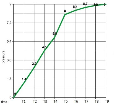
Calculus relies on infinite processes. And the Arduino is a (single thread) computer. So the idea of running a calculus function on an Arduino presents a seemingly impossible scenario. In this article, we’re going to explore the idea of using derivative like techniques with a microcontroller. Let us be reminded that the derivative provides an instantaneous rate of change. Getting an instantaneous rate of change when the function is known is easy. However, when you’re working with a microcontroller and varying analog data without a known function, it’s not so easy. Our goal will be to get an average rate of change of the data. And since a microcontroller is many orders of magnitude faster than the rate of change of the incoming data, we can calculate the average rate of change over very small time intervals. Our work will be based on the fact that the average rate of change and instantaneous rate of change are the same over short time intervals.

Houston, We Have a Problem

In the second article of this series, there was a section at the end called “Extra Credit” that presented a problem and challenged the reader to solve it. Today, we are going to solve that problem. It goes something like this:

We have a machine that adds a liquid into a closed container. The machine calculates the amount of liquid being added by measuring the pressure change inside the container. Boyle’s Law, a very old basic gas law, says that the pressure in a closed container is inversely proportional to the container’s volume. If we make the container smaller, the pressure inside it will go up. Because liquid cannot be compressed, introducing liquid into the container effectively makes the container smaller, resulting in an increase in pressure. We then correlate the increase in pressure to the volume of liquid added to get a calibration curve.

The problem is sometimes the liquid runs out, and gas gets injected into the container instead. When this happens, the machine becomes non-functional. We need a way to tell when gas gets into the container so we can stop the machine and alert the user that there is no more liquid.

One way of doing this is to use the fact that the pressure in the container will increase at a much greater rate when gas is being added as opposed to liquid. If we can measure the rate of change of the pressure in the container during an add, we can differentiate between a gas and a liquid.

Quick Review of the Derivative

Before we get started, let’s do a quick review on how the derivative works. We go into great detail about the derivative here, but we’ll summarize the idea in the following paragraphs.

An average rate of change is a change in position over a change in time. Speed is an example of a rate of change. For example, a car traveling at 50 miles per hour is changing its position at 50 mile intervals every hour. The derivative gives us an instantaneous rate of change. It does this by getting the average rate of change while making the time intervals between measurements increasingly smaller.

Let us imagine a car is at mile marker one at time zero. An hour later, it is at mile marker 50. We deduce that the average speed of the car was 50 miles per hour. What is the speed at mile marker one? How do we calculate that? [Issac Newton] would advise us to start getting the average speeds in smaller time intervals. We just calculated the average speed between mile marker 1 and 50. Let’s calculate the average speed between mile marker’s 1 and 2. And then mile marker’s 1 and 1.1. And then 1 and 1.01, then, 1.001…etc. As we make the interval between measurements smaller and smaller, we begin to converge on the instantaneous speed at mile marker one. This is the basic principle behind the derivative.

Average Rate of Change

We can use a similar process with our pressure measurements to distinguish between a gas and a liquid. The rate of change units for this process is PSI per second. We need to calculate this rate as the liquid is being added. If it gets too high, we know gas has entered the container. First, we need some data to work with. Let us make two controls. One will give us the pressure data for a normal liquid add, as seen in the graph above and to the left. The other is the pressure data when the liquid runs out, shown in the graph on the right. Visually, it’s easy to see when gas gets in the system. We see a surge between time’s T4 and T5.  If we calculate the average rate of change between 1 second time intervals, we see that all but one of them are less that 2 psi/sec. Between time’s 4 and 5 on the gas graph, the average rate of change is 2.2 psi/sec. The next highest change is 1.6 psi/sec between times T2 and T3.

So now we know what we need to do. Monitor the rates of change and error out when it gets above 2 psi/sec.

Our psuedo code would look something like:

pressure = x;
delay(1000);
pressure = y
rateOfChange = (y - x);
if (rateOfChange > 2)
digitalWrite(13, HIGH);  //stop machine and sound alarm

Instantaneous Rate of Change

It appears that looking at the average rate of change over a 1 second time interval is all we need to solve our problem. If we wanted to get an instantaneous rate of change at a specific time, we need to make that 1 second time interval smaller. Let us remember that our microcontroller is much faster than the changing pressure data. This gives us the ability to calculate an average rate of change over very small time intervals. If we make them small enough, the average rate of change and instantaneous rate of change are essentially the same.

Therefore, all we need to do to get our derivative is make the delay smaller, say 50ms. You can’t make it too small, or your rate of change will be zero. The delay value would need to be tailored to the specific machine by some old fashioned trial and error.

Taking the Limit in a Microcontroller?

One thing we have not touched on is the idea of the limit within a microcontroller. Mainly, because we don’t need it. Going back to our car example, if we can calculate the average speed of the car between mile marker one and mile marker 0.0001, why do we need to go though a limiting process? We already have our instantaneous rate of change with the single calculation.

One can argue that the idea behind the derivative is to converge on a single number while going though a limiting process. Is it possible to do this with incoming data of no known function? Let’s try, shall we? We can take advantage of the large gap between the incoming data’s rate of change and the processor’s speed to formulate a plan.

Let’s revisit our original problem and set up an array. We’ll fill the array with pressure data every 10ms. We wait 2 seconds and obtain 200 data points. Our goal is to get the instantaneous rate of change of the middle data point by taking a limit and converging on a single number.

We start by calculating the average rate of change between data points 200 and 150. We save the value to a variable. We then get the rate of change between points 150 and 125. We then compare our result to our previous rate by taking the difference. We continue this process of getting the rate of change between increasingly smaller amounts of time and comparing them by taking the difference. When the difference is a very small number, we know we have converged on a single value.

We then repeat the process in the opposite direction. We calculate the average rate of change between data points 0 and 50. Then 50 and 75. We continue the process just as before until we converge on a single number.

If our idea works, we’ll come up with two values that would look something like 1.3999 and 1.4001 We say our instantaneous rate of change at T1 is 1.4 psi per second. Then we just keep repeating this process.

Now it’s your turn. Think you have the chops to code this limiting process?

The Arduino software environment, including the IDE, libraries, and general approach, are geared toward education. It’s meant as a way to introduce embedded development to newbies. This is a great concept but it falls short when more serious development or more advanced education is required. I keep wrestling with how to address this. One way is by using Eclipse with the Arduino Plug-in. That provides a professional development environment, at least.

The code base for the Arduino is another frustration. Bluntly, the use of setup() and loop() with main() being hidden really bugs me. The mixture of C and C++ in libraries and examples is another irritation. There is enough C++ being used that it makes sense it should be the standard. Plus a good portion of the library code could be a lot better. At this point fixing this would be a monumental task requiring many dedicated developers to do the rewrite. But there are a some things that can be done so let’s see a couple possibilities and how they would be used.

The Main Hack

As mentioned, hiding main() bugs me. It’s an inherent part of C++ which makes it an important to learning the language. Up until now I’d not considered how to address this. I knew that an Arduino main() existed from poking around in the code base – it had to be there because it is required by the C++ standard. The light dawned on me to try copying the code in the file main.cpp into my own code. It built, but how could I be sure that it was using my code and not the original from the Arduino libraries? I commented out setup() and it still built, so it had to be using my version otherwise there’d be an error about setup() being missing. You may wonder why it used my version.

When you build a program… Yes, it’s a “program” not a “sketch”, a “daughter board” not a “shield”, and a “linker” not a “combiner”! Why is everyone trying to change the language used for software development?

When you build a C++ program there are two main stages. You compile the code using the compiler. That generates a number of object files — one for each source file. The linker then combines the compiled objects to create an executable. The linker starts by looking for the C run time code (CRTC). This is the code that does some setup prior to main() being called. In the CRTC there will be external symbols, main() being one, whose code exists in other files.

The linker is going to look in two places for those missing symbols. First, it loads all the object files, sorts out the symbols from them, and builds a list of what is missing. Second, it looks through any included libraries of pre-compiled objects for the remaining symbols. If any symbols are still missing, it emits an error message.

If you look in the Arduino files you’ll find a main.cpp file that contains a main() function. That ends up in the library. When the linker starts, my version of main() is in a newly created object file. Since object files are processed first the linker uses my version of main(). The library version is ignored.

There is still something unusual about main(). Here’s the infinite for loop in main():

	for (;;) {
		loop();
		if (serialEventRun) serialEventRun();
	}

The call to loop() is as expected but why is there an if statement and serialEventRun? The function checks if serial input data is available. The if relies on a trick of the tool chain, not C++, which checks the existence of the symbol serialEventRun. When the symbol does not exist the if and its code are omitted.

Zapping setup() and loop()

Now that I have control over main() I can address my other pet peeve, the setup() and loop() functions. I can eliminate these two function by creating my own version of main(). I’m not saying the use of setup() and loop() were wrong, especially in light of the educational goal of Arduino. Using them makes it clear how to organize an embedded system. This is the same concept behind C++ constructors and member functions. Get the initialization done at the right time and place and a good chunk of software problems evaporate. But since C++ offers this automatically with classes, the next step is to utilize C++’s capabilities.

Global Instantiation

One issue with C++ is the cost of initialization of global, or file, scope class instances. There is some additional code executed before main() to handle this as we saw in the article that introduced classes. I think this overhead is small enough that it’s not a problem.

An issue that may be a problem is the order of initialization. The order is defined within a compilation unit (usually a file) from the first declaration to the last. But across compilation units the ordering is undefined. One time all the globals in file A may be initialized first and the next time those in file B might come first. The order is important when one class depends on another being initialized first. If they are in different compilation units this is impossible to ensure. One solution is to put all the globals in a single compilation unit. This may not work if a library contains global instances.

A related issue occurs on large embedded computer systems, such as a Raspberry Pi running Linux, when arguments from the command line are passed to main(). Environment variables are also a problem since they may not be available until main() executes. Global instance won’t have access to this information so cannot use it during their initialization. I ran into this problem with my robots whose control computer was a PC. I was using the robot’s network name to determine their initial behaviors. It wasn’t available until main() was entered, so it couldn’t be used to initialize global instances.

This is an issue with smaller embedded systems that don’t pass arguments or have environment values but I don’t want to focus only on them. I’m looking to address the general situation that would include larger systems so we’ll assume we don’t want global instances.

Program Class

The approach I’m taking and sharing with you is an experiment. I have done something similar in the past with a robotics project but the approach was not thoroughly analyzed. As often happens, I ran out of time so I implemented this as a quick solution. Whether this is useful in the long run we’ll have to see. If nothing else it will show you more about working with C++.

My approach is to create a Program class with a member run() function. The setup for the entire program occurs in the class constructor and the run() function handles all the processing. What would normally be global variables are data members.

Here is the declaration of a skeleton Program class and the implementation of run():

class Program {
public:
	void run();
	static Program& makeProgram() {
		static Program p;
		return p;
	}

private:
	Program() { }
	void checkSerialInput();
};

void Program::run() {
	for (;;) {
		// program code here
		checkSerialInput();
	}
}

We only want one instance of Program to exist so I’ve assured this by making the constructor private and providing the static makeProgram() function to return the static instance created the first time makeProgram() is called. The Program member function checkSerialInput() handles checking for the serial input as discussed above. In checkSerialInput() I introduced an #if block to eliminate the actual code if the program is not using serial input.

Here is how Program is used in main.cpp:

void arduino_init() {
	init();
	initVariant();
}

int main(void) {
	arduino_init();
	Program& p = Program::makeProgram();
	p.run();
	return 0;
}

The function initArduino() is inlined and handles the two initialization routines required to setup the Arduino environment.

One of the techniques for good software development is to hide complexity and provide a descriptive name for what it does. These functions hide not only the code but, in one case, the conditional compilation.

Redbot Line Follower Project

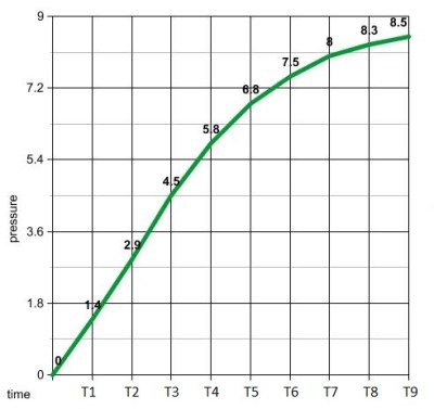
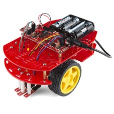
This code experiment uses a Sparkfun Redbot setup for line following. This is a two wheeled robot with 3 optical sensors to detect the line and an I2C accelerometer to sense bumping into objects. The computer is a Sparkfun Redbot Mainboard which is compatible with the Arduino Uno but provides a much different layout and includes a motor driver IC.

This robot is simple enough to make a manageable project but sufficiently complex to serve as a good test, especially when the project gets to the control system software. The basic code for handling these motors and sensors comes from Sparkfun and uses only the basic pin-level Arduino routines. I can’t possibly hack the entire Arduino code but using the Sparkfun code provides a manageable subset for experimenting.

For this article we’ll just look at the controlling the motors. Let’s start with the declaration of the Program class for testing the motor routines:

class Program {
public:
	void run();
	static Program& makeProgram() {
		static Program p;
		return p;
	}

private:
	Program() { }
	static constexpr int delay_time { 2000 };

	rm::Motor l_motor { l_motor_forward, l_motor_reverse, l_motor_pwm };
	rm::Motor r_motor { r_motor_forward, r_motor_reverse, r_motor_pwm };
	rm::Wheels wheels { l_motor, r_motor };

	void checkSerialInput();
};

There is a namespace rm enclosing the classes I’ve defined for the project, hence the rm:: prefacing the class names. On line 11 is something you may not have seen, a constexpr which is new in C++ 11 and expanded in C++14. It declares that delay_time is a true constant used during compilation and will not be allocated storage at run-time. There is a lot more to constexpr and we’ll see it more in the future. One other place I used it for this project is to define what pins to use. Here’s a sample:

constexpr int l_motor_forward = 2;
constexpr int l_motor_reverse = 4;
constexpr int l_motor_pwm = 5;
constexpr int r_motor_pwm = 6;
constexpr int r_motor_forward = 7;
constexpr int r_motor_reverse = 8;

The Motor class controls a motor. It requires two pins to control the direction and one pulse width modulation (PWM) pin to control the speed. The pins are passed via constructor and the names should be self-explanatory. The Wheels class provides coordinated movement of the robot using the Motor instances. The Motor instances are passed as references for the use of Wheels. Here are the two class declarations:

class Motor : public Device {
public:
	Motor(const int forward, const int reverse, const int pwm);

	void coast();
	void drive(const int speed);

	int speed() const {
		return mSpeed;
	}

private:
	void speed(const int speed);

	PinOut mForward;
	PinOut mReverse;
	PinOut mPwm;
	int mSpeed { };
};


class Wheels {
public:
	Wheels(Motor& left, Motor& right) :
			mLeft(left), mRight(right) {
	}

	void move(const int speed) {
		drive(speed, speed);
	}
	void pivot(const int speed) {
		drive(speed, -speed);
	}
	void stop() {
		mLeft.coast();
		mRight.coast();
	}

	void drive(const int left, const int right) {
		mLeft.drive(left);
		mRight.drive(right);
	}

private:
	Motor& mLeft;
	Motor& mRight;
};

The workhorse of Wheels is the function drive() which just calls the Motor drive() functions for each motor. Except for stop(), the other Wheels functions are utilities that use drive() and just make things easier for the developer. The compiler should convert those to a direct call to driver() since they are inline by being inside the class declaration. This is one of the interesting ways of using inline functions to enhance the utility of a class without incurring any cost in code or time.

The run() method in Program tests the motors by pivot()ing first in one direction and then the other at different speeds. A pivot() rotates the robot in place. Once the speed is set it continues until changed so the delay functions simply provide a little time for the robot to turn. Here’s the code:

void Program::run() {
	for (;;) {
		wheels.pivot(50);
		delay (delay_time);

		wheels.pivot(-100);
		delay(delay_time);

		checkSerialInput();
		if (serialEventRun) {
		}
	}
}

Wrap Up

The Redbot project is an interesting vehicle for demonstrating code techniques. The current test of the motor routines demonstrates how to override the existing Arduino main(). Even if you don’t like my approach with Program, the flexibility of using your own main() may come in handy for your own projects. The next article is going to revisit this program using templates.

THE EMBEDDING C++ PROJECT

Over at Hackaday.io, I’ve created an Embedding C++ project. The project will maintain a list of these articles in the project description as a form of Table of Contents. Each article will have a project log entry for additional discussion. Those interested can delve deeper into the topics, raise questions, and share additional findings.

The project also will serve as a place for supplementary material from myself or collaborators. For instance, someone might want to take the code and report the results for other Arduino boards or even other embedded systems. Stop by and see what’s happening.

If you don’t have a Raspberry Pi Zero right now, you’re not getting one for Christmas. Who would have thought a $5 Linux computer would have been popular, huh? If you’re looking for a new microcontroller platform you can actually buy, the Arduino / Genuino 101 is available in stores. This was released a few months ago, but it still looks pretty cool: DSP, BTLE, and a six-axis sensor.

If you don’t know [David], the Swede, you should. He’s the guy that launched a glider from a high altitude balloon and is one of the biggest advocates of tricopters. Now he bought an airplane wing for his front yard. It was an old Swedish air force transport aircraft being broken up for scrap. Simply awesome.

Chocolate chips. Now that the most obvious pun is out of the way, here’s how you make DIP8 cookie cutters.

[Barb] is over at the Crash Space hackerspace in LA, and she has a YouTube channel that goes over all her creations. This week, it’s a layered wood pendant constructed out of many layers of veneer. Take note of the 3M 77 spray glue used for the lamination and the super glue used as a clear, hard finish.

Star Wars was released and we have a few people digging through the repertoire to see what [John Williams] lifted for the new movie. Here’s musical Tesla coils playing the theme for the Force.

Flickr gives you a full gigabyte of storage, but only if you upload JPEGs, GIFs, and PNGs. That doesn’t prevent you from using Flickr as your own cloud storage.

We know two things about [Hans Fouche]: he lives in South Africa and he has a gigantic 3D printer. His latest creation is an acoustic guitar. It may not sound great, but that’s the quality of the recording. It may not play great, but he can fix that with some acetone vapor. It would be very interesting to see 3D printing used in a more traditional lutherie context; this printer could easily print molds and possibly even something to bend plywood tops.

Starting in 1990, [deater] would make a yearly Christmas-themed demo on his DOS box. You can really see the progression of technology starting with ANSI art trees written in BASIC, to an EGA graphical demo written with QBASIC to the last demo in 96 made with VGA, and SoundBlaster effects written in Turbo Pascal and asm.

The language C++ is big. There is no doubting that. One reason C++ is big is to allow flexibility in the technique used to solve a problem. If you have a really small system you can stick to procedural code encapsulated by classes. A project with a number of similar but slightly different entities might be best addressed through inheritance and polymorphism.

A third technique is using generics, which are implemented in C++ using templates. Templates have some similarities with #define macros but they are a great deal safer. The compiler does not see the code inserted by a macro until after it has been inserted into the source. If the code is bad the error messages can be very confusing since all the developer sees is the macro name. A template is checked for basic syntax errors by the compiler when it is first seen, and again later when the code is instantiated. That first step eliminates a lot of confusion since error messages appear at the location of the problem.

Templates are also a lot more powerful. They actually are a Turing complete language. Entire non-trivial programs have been written using templates. All the resulting executable does is report the results with all the computation done by the compiler. Don’t worry, we aren’t going there in this article.

Template Basics

You can use templates to create both functions and classes. The way this is done is quite similar for both so let’s start with a template function example:

template<typename T, int EXP = 2>
T power(const T value, int exp = EXP) {
	T res { value };
	for (; exp > 1; --exp) {
		res *= value;
	}
	return res;
}

This is a template function for raising value by the integer exponent, exp. The keyword template is followed in angle brackets by parameters. A parameter is specified using either typename or class followed by a name, or by an integer data type followed by a name. You can also use a function or class as a template parameter but we won’t look at that usage.

The name of a parameter is used within the body of the class or function just as you would use any other type, or value. Here we use T as the type name for the input and return values of the function. The integer EXP is used to set a default value of 2 for the exponent, i.e. making power calculate the square.

When the compiler instantiates a template function or class, it creates code that is the same as a handwritten version. The data types and values are inserted as text substitutions. This creates a new version typed by the actual arguments to the parameters. Each different set of arguments creates a new function or type. For example, an instance of power() for integers is not the same as power() for floats. Similarly, as we’ll see in a moment, a class Triple for integers is not the same as one for float. Each are distinct types with separate code.

Since power() is a template function it will work directly for any numeric data type, integer or floating point. But what if you want to use it with a more complex type like the Triple class from the last article? Let’s see.

Using Templates

Here’s the declaration of Triple reduced to only what is needed for this article:

class Triple {
public:
	Triple(const int x, const int y, const int z);
	Triple& operator *=(const Triple& rhs);

	int x() const;
	int y() const;
	int z() const;

private:
	int mX { 0 };	// c++11 member initialization
	int mY { 0 };
	int mZ { 0 };
};

I switched the plus equal operator to the multiple equal operator since it is needed by the power() function.

Here is how the power() function is used for integer, float, and our Triple data types:

int p = power(2, 3);
float f = power(4.1, 2);

Triple t(2, 3, 4);
Triple res = power(t, 3);

The only requirement for using a user defined data type (UDT) like Triple with power() is the UDT must define an operator=*() member function.

Template Classes

Assume you’ve been using Triple in a project for awhile with integer values. Now a project requirement needs it for floating point values. The Triple class code is all debugged and working, and more complex than what we’ve seen here. It’s not a pleasant thought to create a new class for float. There are also hints that a long or double version might be needed.

With not much work Triple can be converted to a generic version as a template class. It’s actually fairly straightforward. Begin with the template declaration just as with the function power() and replace all the declarations of int with T. Also check member function arguments for passing parameters by value. They may need to be changed to references to more efficiently handle larger data types or UDTs. I changed the constructor parameters to references for this reason.

Here is Triple as a template class:

template<typename T>
class Triple {
public:
	Triple(const T& x, const T& y, const T& z);
	Triple& operator *=(const Triple& rhs);

	T x() const;
	T y() const;
	T z() const;

private:
	T mX { 0 };	// c++11 member initialization
	T mY { 0 };
	T mZ { 0 };
};

Not a lot of difference. Here’s how it could be used:

Triple<int> ires = power(Triple { 2, 3, 4 }, 3);
Triple fres = power(Triple(1.2F, 2.2, 3.3)); // calc square
Triple dres = power(Triple(1.2, 2.2, 3.3));// calc square
Triple lres = power(Triple(1, 2, 3.3), 2);

Unfortunately, the new flexibility comes at the cost of telling the template the data type to use for Triple. That is done by putting the data type inside brackets following the class name. If that is a hassle you can always use typedef or the new using to create an alias:

using TripleInt = Triple;
TripleInt ires = power(Triple { 2, 3, 4 }, 3);

Creating a template class like this saves debugging and maintenance costs overall. Once the code is working, it works for all related data types. If a bug is found and fixed, it’s fixed for all versions.

Template Timing and Code Size

The code generated by a template is exactly the same code as a handwritten version of the same function or class. All that changes between versions is the data type used in the instantiation. Since the code is the same as the handwritten version, the timing is going to be the same. Therefore there is no need to actually test timing. Phew!

Templates are Inline Code

Templates are inherently inline code. That means every time you use a template function or a template class member function the code is duplicated inline. Each instance with a different data type creates its own set of code, but that will be no more than if you’d written a class for each data type. There can be savings using template classes since member functions are not instantiated if they are not used. For example, if the Triple class getter functions – x(), y(), z() – are never used, their code is not instantiated. They would be for a regular class, although a smart linker might drop them from the executable.

Consider the following use of power() and Triple:

int i1 = power(2, 3);
int i2 = power(3, 3);
Triple t1 = power(Triple(1, 2, 3), 2);

This creates two inline integer versions of power even though both are instantiated for the same data type. Another instance is created for the Triple version. A single copy of the Triple class is created because the data type is always int.

Here we’re relying on implicit instantiation. That means we’re letting the compiler determine when and where the code is generated. There is also explicit instantiation that allows the developer to specify where the code is produced. This takes a little effort and knowledge of which data types are used for the templates.

Generally, implicit instantiation means inline function code with the possibility of duplication of code. Whether that matters depends on the function. When a function, not an inline function, is called there is overhead in invocation. The parameters to the function are pushed onto the stack along with the housekeeping information. When the function returns those operations are reversed. For a small function the invocation may take more code than the function’s body. In that case, inlining the function is most effective.

The power() function used here is interesting because the function’s code and the code to invoke it on an Uno are similar in size. Of course, both vary depending on the data type since large data types require more stack manipulation. On a Arduino Uno, calling power() with an int takes more code than the function. For float, the call is slightly larger. For Triple, the code to invoke is a good piece larger. On other processors the calling power() could be different. Keep in mind that power() is a really small function. Larger functions, especially member functions, are typically going to outweigh the cost to call them.

Specifying where the compiler generates the code is an explicit instantiation. This will force an out-of-line call with the associated overhead. In a source file you tell the compiler which specializations you need. For the test scenario we want them for int and Triple:

template int power(int, int);
template Triple<int> power(Triple<int>, int);

The compiler will create these in the source file. Then, as with any other function, you need to create an extern declaration. This tells the compiler to not instantiate them as inline. These declarations are just the same as above, only with extern added:

extern template int power(int, int);
extern template Triple power(Triple, int);

Scenario for Testing Code Size

It took me a bit to create a test scenario for demonstrating the code size differences between these two instantiations. The problem is the result from the power() function must be used later in the code or the compiler optimizes the call away. Adding code to use the function changes the overall code size in ways that are not relevant to the type of instantiation. That makes comparisons difficult to understand.

I finally settled on creating a class, Application, with data members initialized using the power() function. Adding data members of the same or different types causes minimal overall size changes so the total application code size closely reflects the changes only due to the type of instantiation.

Here is the declaration of Application:

struct Application {
public:
	Application(const int value, const int exp);

	static void loop() {
	}

	int i1;
	int i2;
	int i3;
	Triple t1;
	Triple t2;
	Triple t3;
};

and the implementation of the constructor:

Application::Application(int value, const int exp) :
		i1 { power(value++, exp) }, //
				i2 { power<int, 3="">(value++) }, // calcs cube
				i3 { power(value++, exp) }, //

				t1 { power(Triple(value++, 2, 3)) }, // calcs square
				t2 { power(Triple(value++, 4, 5), exp) }, //
				t3 { power(TripleInt(value++, 2, 3), exp) } //
{
}

The minimum application for an Arduino has just an empty setup and loop() functions which takes 450 bytes on a Uno. The loop() used for this test is a little more than minimum but it only creates an instance of Application and calls its loop() member function:

void loop() {
	rm::Application app(2, 3);
	rm::Application::loop();	// does nothing
}

Code Size Results

Here are the results for various combinations of implicit and explicit instantiation with different numbers of class member variables:

The first columns specify how many variables were included in the Application class. The columns under Uno and Due are the code size for those processors. They show the size for implicit instantiation, explicit instantiation of power() for just the Triple class, and explicit instantiation for both int and Triple data types.

The code sizes are dependent on a number of factors so can only provide a general idea of the changes when switching from implicit to explicit template instantiation. Actual results depend on the tool chains compiler and linker. Some of that occurs here using the Arduino’s GCC tool chain.

In all the cases with the Uno where one variable is used, the code size increases with explicit instantiation. In this case the function’s code plus the code for calling the function is, as expected, greater than the inline function’s code.

Now look at the Uno side of the table where there are 2 integers and 2 Triples, i.e. the fourth line. The first two code sizes remain the same at 928 bytes. The compiler optimized the code for the two Triples() by creating power() out-of-line without being told to do it explicitly. In the third column there is a decrease in code size when the integer version of power() is explicitly instantiated. It did the same a couple of lines below that when there are only the 2 Triples. These were verified by examing the assembly code running objdump on the ELF file.

In general, the Due’s code size did not improve with explicit instantiation. The larger word size of the Due requires less code to call a function. It would take a function larger than power() to make explicit instantiation effective in this scenario.

As I mentioned, don’t draw too many conclusions for these code sizes. I repeatedly needed to check the content of the ELF file using objdump to verify my conclusions. As a case in point, look at the Due side, with 2 integers and a Triple, with the two code sizes of 10092. They’re just coincidence. In one the integer version of power() is inlined and in the other, explicitly out-of-lined. The same occurs on the first line under Uno where there are just two integers and no Triples.

You can find other factors influencing code size. When three Triples are involved the compiler lifts the multiplication code from power(), but not the entire function. This isn’t because power() is a template function but just a general optimization, i.e. lifting code from inside a loop.

Wrap Up

Templates are a fascinating part of C++ with extremely powerful capabilities. As mentioned above, you can write an entire program in templates so the compiler actually does the computation. The reality is you probably are not going to be creating templates in every day programming. They are better suited for developing libraries and general utilities. Both power() and Triple fall into, or are close to, that category. This is why the C++ libraries consist of so many template classes. Creating a library requires attention to details beyond regular coding.

It’s important to understand templates even if you don’t write them. We’ve discussed some of the implications of usage and techniques for making optimal use of templates because they are an inherent part of the language. With them being such a huge part of C++ we’ll come back to them again to address places where they can be used.

The Embedding C++ Project

Over at Hackaday.io, I’ve created an Embedding C++project. The project will maintain a list of these articles in the project description as a form of Table of Contents. Each article will have a project log entry for additional discussion. Those interested can delve deeper into the topics, raise questions, and share additional findings.

The project also will serve as a place for supplementary material from myself or collaborators. For instance, someone might want to take the code and report the results for other Arduino boards or even other embedded systems. Stop by and see what’s happening.

There’s a new documentary series on Al Jazeera called Rebel Geeks that looks at the people who make the stuff everyone uses. The latest 25-minute part of the series is with [Massimo], chief of the arduino.cc camp. Upcoming episodes include Twitter co-creator [Evan Henshaw-Plath] and people in the Madrid government who are trying to build a direct democracy for the city on the Internet.

Despite being a WiFi device, the ESP8266 is surprisingly great at being an Internet of Thing. The only problem is the range. No worries; you can use the ESP as a WiFi repeater that will get you about 0.5km further for each additional repeater node. Power is of course required, but you can stuff everything inside a cell phone charger.

I’ve said it before and I’ll say it again: the most common use for the Raspberry Pi is a vintage console emulator. Now there’s a Kickstarter for a dedicated tabletop Raspi emulation case that actually looks good.

Pogo pins are the go-to solution for putting firmware on hundreds of boards. These tiny spring-loaded pins give you a programming rig that’s easy to attach and detach without any soldering whatsoever. [Tom] needed to program a few dozen boards in a short amount of time, didn’t have any pogo pins, and didn’t want to solder a header to each board. The solution? Pull the pins out of a female header. It works in a pinch, but you probably want a better solution for a more permanent setup.

Half of building a PCB is getting parts and pinouts right. [Josef] is working on a tool to at least semi-automate the importing of pinout tables from datasheets into KiCad. This is a very, very hard problem, and if it’s half right half the time, that’s a tremendous accomplishment.

Last summer, [Voja] wrote something for the blog on building enclosures from FR4. Over on Hackaday.io he’s working on a project, and it’s time for that project to get an enclosure. The results are amazing and leave us wondering why we don’t see this technique more often.

What is an embedded system? The general definition is a computer system dedicated to a specific purpose, i.e. not a general purpose system usable for different tasks. That is a very broad definition. I was just skimming the C++ coding guidelines for the Joint Strike Fighter. That’s a pretty big embedded system and the first DOD project that allowed C++! When you use an ATM to get money you’re using an embedded system. Those are basically hardened PCs. Then at the small end we have all the Internet of Things (IoT) gadgets.

The previous articles about embedding C++ discussing classes, virtual functions, and macros garnered many comments. I find both the positive and critical comments rewarding. More importantly, the critical comments point me toward issues or questions that need to be addressed, which is what got me onto the topic for this article. So thank you, all.

Let’s take a look at when embedded systems should or should not use C++, taking a hard look at the claim that there may be hidden activities ripe to upset your carefully planned code execution.

Limits of Embedded Development Boards

Embedded systems are often thought of as having limited resources, e.g. memory, processing power. Having real-time constraints is another requirement frequently brought up. While those do occur in embedded systems they are not defining characteristics.

At some point a processor or memory limits preclude using C++, and often even C. Vendors might resort to a restricted version of C on some processors to provide a high-level language capability, an effort that would be silly for C++.

But we’ve not hit the limit on the boards used in these articles. We see with the Arduino Uno and its relatives that C++ is usable. The Uno is restricted to a subset of C++, in part because the developers did not have a C++ standard library available. (If you really want one, there are ports of the STL for the Uno.) The compiler in the Uno toolset supports C++11 and there is some support for C++14, but I haven’t explored the latter to know what is usable. There are capabilities in C++11, and C+14, that improve C++ use in embedded systems.

The Due, a larger Arduino board I’ve used to contrast with the Uno, does have the full standard library. Switch over to the Raspberry Pi, or equivalents, where you not only get the GCC toolset but can run Eclipse on the board, and it feels like the sky’s the limit.

Should You C++?

While all the above is valid, it misses a critical point. The issue isn’t whether you can use C++ on the smaller systems but whether solving the problem needs C++’s capabilities. What I’m suggesting is changing the question from “Can you use C++?” to “Should you use C++?”

We’ve addressed some of the really basic objections to using C++. Code bloat is not the great explosion folks imagine. Virtual functions are not super slow. But the comments raise other issues. One comment advised against using C++ because of the hidden activities. Specifically mentioned were copy constructors, side effects, hidden allocation, and unexpected operations.

What is a copy constructor, and why do we need one? It’s a constructor that makes a copy of an existing instance. Any time a copy is made the copy constructor is called. Recall that all constructors initialize instances so they are ready to be used.

A copy constructor is required if you pass a parameter by value. That’s a copy. Returning a value from a function causes a copy, although a decent compiler will optimize it away. Assignment also involves making a copy.

With built in types the cost of a copy is low, except maybe if you are using long doubles at 16 bytes a value. For large data structures a copy can be expensive and can be tricky. Rather than bemoan that C++ does copies, we need to recognize they are a necessity. That recognition means we can work to avoid them and get them right when they are needed.

One way to avoid copies is to pass structures by reference. In C, passing by pointer is a pass by reference. C++ allows that and introduces the reference operator. The reference operator is not just syntactic sugar. For example, references eliminate the dangling pointer problem since you cannot have a null reference.

Which brings up the ownership problem with pointers and the questions they raise for data structure copies. Quite frequently, even in C++, a data structure contains a pointer to another data structure. When you make a copy who owns the structure at the end of the pointer? Do you copy the pointer or the data? If you just copy the pointer you are sharing data between the two copies. One copy can modify the data in the other copy. That is usually not a good thing. Copying the data might be expensive. Also, who ultimately decides when the target of a pointer is deleted, or even if it should be deleted?

C++ doesn’t introduce a problem with copy constructors; it highlights a requirement that needs to be addressed, sometimes by looking to the problem requirements. What is needed by the solution when a copy is made?

Copying Data

In my robotics work I use an inertial measurement unit (IMU) to help track position and bearing, the robot’s pose. Inside the IMU are an accelerometer, a gyroscope, and a compass. The accelerometer and gyroscope both provide data as a triple of data, i.e. measurements in x, y, and z axis. There are a number of operations that need to be done on that data to make it usable, many more than we want to look at here. But we can look at how to handle this triple of data and to add a triple of values together. This is done with the gyroscope since it reports the angular rate of change per unit of time. By accumulating those readings you can obtain, theoretically, the bearing of the robot.

C++ Implementation

Here’s the declaration of the class Triple and the overloaded addition operator:

class Triple {
public:
	Triple() = default; // C++11 use default constructor despite other constructors being declared
	Triple(const Triple& t);	// copy constructor so we can track usage
	Triple(const int x, const int y, const int z);

	const Triple& operator +=(const Triple& rhs);

	int x() const;
	int y() const;
	int z() const;
private:
	int mX { 0 };	// C++11 member initialization
	int mY { 0 };
	int mZ { 0 };
};

inline Triple operator+(const Triple& lhs, const Triple& rhs);

I’m using a number of C++11 features here. They’re marked, and the implications for most are obvious if you are familiar with earlier versions of C++. The line with Triple() = default; probably isn’t obvious. It requests that the compiler generate the default constructor. Without it we couldn’t create a variable with no arguments on the constructor: Triple t3;. Normally the default constructor is only created by the compiler when no other constructors are defined. Since Triple has two other constructors there would be no default constructor. I requested one using the notation so variables could be created without arguments.

The next constructor, Triple(const Triple& t), is the copy constructor. It is not needed for this class since C++ would have generated one by default that would have worked fine for this simple class. I created it to show how one works and illustrate where it is invoked. This uses a new C++11 feature where a constructor can invoke another constructor to handle the initialization. This came into being to avoid code duplication, which often led to errors, or the use of a class member to perform initialization.

The final constructor allows us to initialize a Triple with three values. Those three values are stored in the data members of the class.

The next function overloads the plus equals operator. It turns out that the most effective way to implement the actual addition operator, seen a few lines below, is to first implement this operator.

The remaining functions are getters because they allow us to get data from the class. Some classes also have setters that allow setting class values. We don’t want them in Triple.

Here are the implementations of the arithmetic operators:

inline const Triple& Triple::operator +=(const Triple& rhs) {
	mX += rhs.mX;
	mY += rhs.mY;
	mZ += rhs.mZ;
	return *this;
}

inline Triple operator+(const Triple& lhs, const Triple& rhs) {
	Triple left { lhs };
	left += rhs;
	return left;
}

The first operator is straightforward; it simply applies the plus equal operator to each value in the class and returns the instance as a reference. This operator modifies the data in the calling object so the returned reference is valid.

The addition operator uses the plus equal operator in its implementation. Here is where the copy constructor comes into play. We have to create a new object to hold the result so one is created from the lhs value. That’s a copy.

The rhs is added to the new object using plus equal operator and the result returned by value, not by reference. The return is another copy. It cannot be returned by reference because the result object, left, was created inside the function.

There are two possible copies in any arithmetic operator. However, C++ in the standard specifically allows compilers to optimize away the copy for the return value. This is the return value optimization. You’re welcome to try adjusting the code, but there is no way you can avoid creating a copy or two somewhere during this operation.

This code will run on an Arduino, but I created it and ran it on Linux so I could step through the operations to verify where the copy constructor was called and where it wasn’t.

How do you use this? Pretty much the same as any arithmetic operation:

	Triple t1 { 1, 2, 3 };
	Triple t2 { 10, 20, 30 };

	Triple t3 { t1 + t2 };

C Implementation

What would a similar implementation look like in C? How about this:

struct Triple {
	int mX;
	int mY;
	int mZ;
};

void init(struct Triple* t, const int x, const int y, const int z) {
	t->mX = x;
	t->mY = y;
	t->mZ = z;
}
struct Triple add(struct Triple* lhs, struct Triple* rhs) {
	struct Triple result;
	result.mX = lhs->mX + rhs->mX;
	result.mY = lhs->mY + rhs->mY;
	result.mZ = lhs->mZ + rhs->mZ;
	return result;
}

Overall it looks shorter and neater. The struct Triple contains the three data items for the axis. The routine init sets them to user specified values. The add function adds two Triples and returns the result. The add routine avoids initializing result because we know its content will be overwritten by the addition operations. That’s a bit of a savings for C. There is still a copy when the function returns the value. You just don’t have any control of how that copy is done. In this simple situation it doesn’t matter but with a more complicated data structure, say, one with pointers, the copy might be more challenging. We’d probably need to resort to an output parameter using pass by reference with pointers instead of a return value.

Here is how it is used:

	struct Triple t1;
	init(&t1, 1, 2, 3);

	struct Triple t2;
	init(&t2, 10, 20, 30);

	struct Triple t3 = add(&t1, &t2);

Two values are created and initialized and then added. Simple, but you’ve got to remember to take the addresses of the structures and to assure the init routine is only called once.

Consider how the two different versions would look if you implemented a complicated expression. I’ll just say I know which I would prefer.

Wrap Up

I didn’t start this article intending to do a direct comparison between the two languages. I only wanted to illustrate that the copy constructor is, if you insist, a necessary evil. Copies occur in multiple places in both C++ and C. They become critical to understand in C++ when using user defined data types, i.e. classes. Copying in C is less obvious but still necessary.

Since I didn’t intend to make a comparison, I don’t have code size or timings for the two versions. As I pointed out and demonstrated in the article on virtual functions, comparing these simple examples on those parameters is often misleading. A C++ capability is used to solve a problem, not just as an exercise of the language features. Only if an equivalent solution in C is created is a comparison valid.

The Embedding C++ Project

Over at Hackaday.io, I’ve created an Embedding C++project. The project will maintain a list of these articles in the project description as a form of Table of Contents. Each article will have a project log entry for additional discussion. Those interested can delve deeper into the topics, raise questions, and share additional findings.

The project also will serve as a place for supplementary material from myself or collaborators. For instance, someone might want to take the code and report the results for other Arduino boards or even other embedded systems. Stop by and see what’s happening.