Direct-digital synthesis (DDS) is a sample-playback technique that is useful for adding a little bit of audio to your projects without additional hardware. Want your robot to say ouch when it bumps into a wall? Or to play a flute solo? Of course, you could just buy a cheap WAV playback shield or module and write all of the samples to an SD card. Then you wouldn’t have to know anything about how microcontrollers can produce pitched audio, and could just skip the rest of this column and get on with your life.

But that’s not the way we roll. We’re going to embed the audio data in the code, and play it back with absolutely minimal additional hardware. And we’ll also gain control of the process. If you want to play your samples faster or slower, or add a tremolo effect, you’re going to want to take things into your own hands. We’re going to show you how to take a single sample of data and play it back at any pitch you’d like. DDS, oversimplified, is a way to make these modifications in pitch possible even though you’re using a fixed-frequency clock.

The same techniques used here can turn your microcontroller into a cheap and cheerful function generator that’s good for under a hundred kilohertz using PWM, and much faster with a better analog output. Hackaday’s own [Bil Herd] has a nice video post about the hardware side of digital signal generation that makes a great companion to this one if you’d like to go that route. But we’ll be focusing here on audio, because it’s easier, hands-on, and fun.

We’ll start out with a sample of the audio that you’d like to play back — that is some data that corresponds to the voltage level measured by a microphone or something similar at regular points in time. To play the sample, all we’ll need to do is have the microcontroller output these voltages back at exactly the same speed. Let’s say that your “analog” output is via PWM, but it could easily be any other digital-to-analog converter (DAC) of your choosing. Each sample period, your code looks up a value and writes it out to the DAC. Done!

(In fact, other than reading the data from an SD card’s filesystem, and maybe having some on-board amplification, that’s about all those little WAV-player units are doing.)

Pitch Control

In the simplest example, the sample will play back at exactly the same pitch it was recorded if the sample playback rate equals the input sampling rate. You can make the pitch sound higher by playing back faster, and vice-versa. The obvious way to do this is to change the sample-playback clock. Every period you play back one the next sample, but you change the time between samples to give you the desired pitch. This works great for one sample, and if you have infinitely variable playback rates available.

But let’s say that you want to take that sample of your dog barking and play Beethoven’s Fifth with it. You’re going to need multiple voices playing the sample back at different speeds to make the different pitches. Playing multiple pitches in this simplistic way, would require multiple sample-playback clocks.

Here’s where DDS comes in. The idea is that, given a sampled waveform, you can play nearly any frequency from a fixed clock by skipping or repeating points of the sample as necessary. Doing this efficiently, and with minimal added distortion, is the trick to DDS. DDS has its limits, but they’re mostly due to the processor you’re using. You can buy radio-frequency DDS chips these days that output very clean sampled sine waves up to hundreds of megahertz with amazing frequency stability, so you know the method is sound.

Example

Let’s make things concrete with a simplistic example. Say we have a sample of a single cycle of a waveform that’s 256 bytes long, and each 8-bit byte corresponds to a single measured voltage at a point in time. If we play this sample back at ten microseconds per sample we’ll get a pitch of 1 / (10e-06 * 256) = 390.625 Hz, around the “G” in the middle of a piano.

Imagine that our playback clock can’t go any faster, but we’d nonetheless like to play the “A” that’s just a little bit higher in pitch, at 440 Hz. We’d be able to play the “A” if we had only sampled 227 bytes of data in the first place: 1 / (10e-06 * 227) = 440.53, but it’s a little bit late to be thinking of that now. On the other hand, if we just ignored 29 of the samples, we’d be there. The same logic works for playing lower notes, but in reverse. If some samples were played twice, or even more times, you could slow down the repetition rate of the cycle arbitrarily.

In the skipping-samples case, you could just chop off the last 29 samples, but that would pretty seriously distort your waveform. You could imagine spreading the 29 samples throughout the 256 and deleting them that way, and that would work better. DDS takes this one step further by removing different, evenly spaced samples with each cycle through the sampled waveform. And it does it all through some simple math.

The crux is the accumulator. We’ll embed the 256 samples in a larger space — that is we’ll create a new counter with many more steps so that each step in our sample corresponds to many numbers in our larger counter, the accumulator. In my example code below, each of the 256 steps gets 256 counts. So to advance one sample per period, we need to add 256 to the larger counter. To go faster, you add more than 256 each period, and to go slower, add less. That’s all there is to it, except for implementation details.

In the graph here, because I can’t draw 1,024 tick marks, we have 72 steps in the accumulator (the green outer ring) and twelve samples (inner, blue). Each sample corresponds to six steps in the accumulator. We’re advancing the accumulator four steps per period (the red lines) and you can see how the first sample gets played twice, then the next sample played only once, etc. In the end, the sample is played slower than if you took one sample per time period. If you take more than six steps in the increment, some samples will get skipped, and the waveform will play faster.

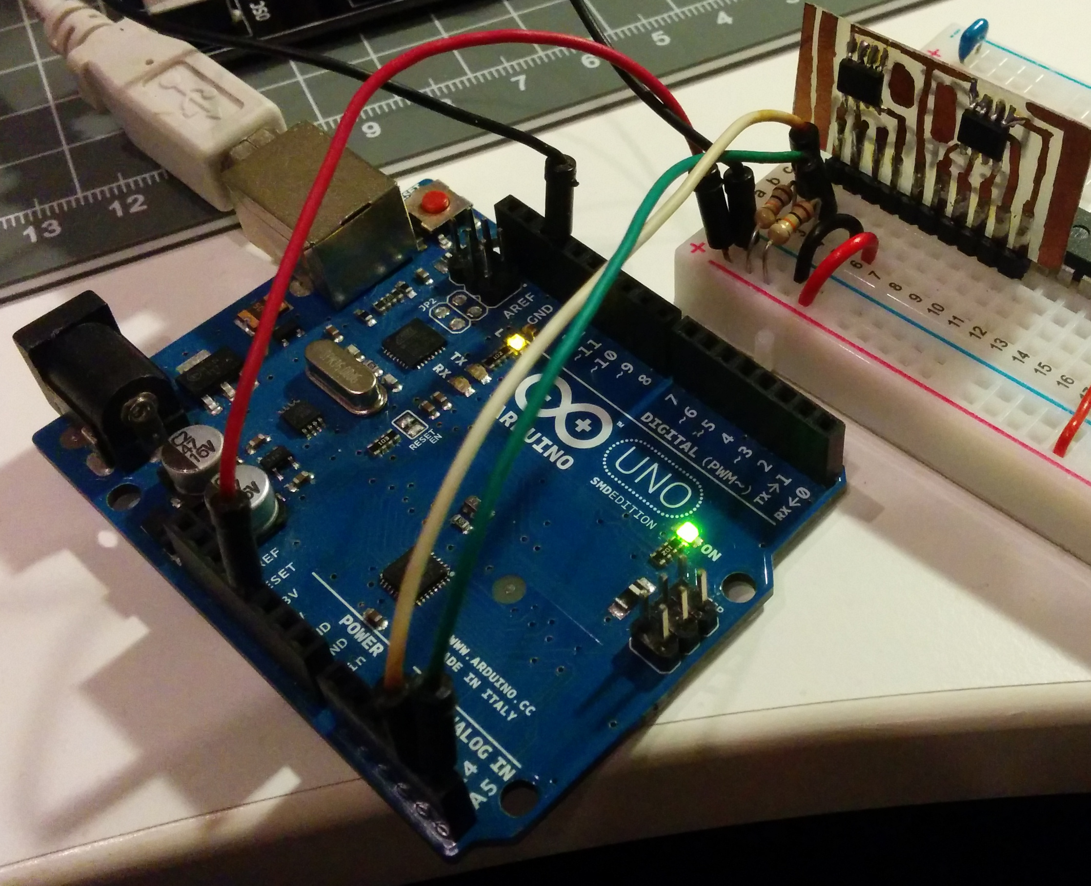
Implementation and Build

So let’s code this up and flash it into an Arduino for testing. The code is up at GitHub for you to follow along. We’ll go through three demos: a basic implementation that works, a refined version that works a little better, and finally a goofy version that plays back single samples of dogs barking.

In overview, we’ll be producing the analog output waveforms using filtered PWM, and using the hardware-level PWM control in the AVR chip to do it. Briefly, there’s a timer that counts from 0 to 255 repeatedly, and turns on a pin at the start and turns it off at a specified top value along the way. This lets us create a fast PWM signal with minimal CPU overhead, and it uses a timer.

We’ll use another timer that fires off periodically and runs some code, called an interrupt service routine (ISR), that loads the current sample into the PWM register. All of our DDS code will live in this ISR, so that’s all we’ll focus on.

If this is your first time working directly with the timer/counters on a microcontroller, you’ll find some configuration code that you don’t really have to worry about. All you need to know is that it sets up two timers: one running as fast as possible and controlling a PWM pin for audio output, and another running so that a particular chunk of code is called consistently, 24,000 times per second in this example.

So without further ado, here’s the ISR:

struct DDS {
    uint16_t increment;
    uint16_t position;
    uint16_t accumulator;
    const int8_t* sample;   /* pointer to beginning of sample in memory */
};
volatile struct DDS voices[NUM_VOICES];

ISR(TIMER1_COMPA_vect) {
    int16_t total = 0;

    for (uint8_t i = 0; i < NUM_VOICES; i++) {
        total += (int8_t) pgm_read_byte_near(voices[i].sample + voices[i].position);

        /* Take an increment step */
        voices[i].accumulator += voices[i].increment;
        voices[i].position += voices[i].accumulator / ACCUMULATOR_STEPS;
        voices[i].accumulator = voices[i].accumulator % ACCUMULATOR_STEPS;
        voices[i].position = voices[i].position % SAMPLE_LENGTH;
    }

    total = total / NUM_VOICES;
    OCR2A = total + 128; // add in offset to make it 0-255 rather than -128 to 127
}

The first thing the code does is to define a (global) variable that will hold the state of each voice for as many voices as we want, defined by NUM_VOICES. Each voice has an increment which determines how many steps to take in the accumulator per sample output. The position keeps track of exactly which of the 256 samples in our waveform data is currently playing, and the accumulator keeps track of the rest. Here, we’re also allowing for each voice to play back a different waveform table from memory, so the code needs to keep track of the address where each sample begins. Changing which sample gets played back is as simple as pointing this variable to a different memory location, as we’ll see later. For concreteness, you can imagine this sample memory to contain the points in a sine wave, but in practice any repetitive waveform will do.

So let’s dive into the ISR, and the meat of the routine. Each update cycle, the sum of the output on the different voices is calculated in total. For each voice, the current sample is read from memory, added to the total and then incremented to the next step. Here we get to see how the accumulator works. The increment variable is added to the accumulator. When the accumulator is larger than the number of steps per sample, the position variable gets moved along. Next, the accumulator is shrunk back down to just the remainder of the un-accounted-for values using the modulo operator, and the sample position is wrapped around if necessary with another modulo.

Division?? Modulo??

If you’ve worked with microcontrollers before, alarm bells may be going off in your head right now. The AVR doesn’t have a built-in division routine, so that could take a lot of CPU power. And the modulo operator is even worse. That is, unless the divisor or modulo are powers of two. In those cases, the division is the same as shifting the binary number to the right by the number of bits in the power of two.

A similar operation makes the modulo tolerable. If, for instance, you want a number to be modulo eight, you can simply drop all of the binary bits that correspond to values eight and higher. So, x % 8 can be implemented as x & 0b00000111 where this logical-ANDing just keeps the least-significant three bits. If you’re not in tune with your inner bit-flipper, this can be viewed as a detail — but just know that division and modulo aren’t necessarily bad news if your compiler knows how to implement them efficiently when you choose powers of two for the divisors.

And that gets us to the end of the routine. The sample values were added together, so now they need dividing by the number of voices and centering around the mid-point to fit inside the 8-bit range that the PWM output register requires. As soon as this value is loaded into memory, the PWM hardware will take care of outputting the right waveform on its next cycle.

Refinements

The ISR above is already fairly streamlined. It’s avoided the use of any if statements that would otherwise slow it down. But it turns out we can do better, and this optimized form is often the way you’ll see DDS presented. Remember, we’re running this ISR (in this example) 24,000 times per second — any speedup inside the ISR makes a big difference in overall CPU usage.

The first thing we’ll do is make sure that we have only 256 samples. That way, we can get rid of the line where we limit the sample index to being within the correct range simply by using an 8-bit variable for the sample value. As long as the number of bits in the sample index matches the length of the sample, it will roll over automatically.

We can use the same logic to merge the sample and accumulator variables above into a single variable. If we have an 8-bit sample and an 8-bit accumulator, we combine them into a 16-bit accumulator where the top eight bits correspond to the sample location.

struct DDS {
    uint16_t increment;
    uint16_t accumulator;
    const int8_t* sample;   /* pointer to beginning of sample in memory */
};
volatile struct DDS voices[NUM_VOICES];

ISR(TIMER1_COMPA_vect) {
    int16_t total = 0;

    for (uint8_t i = 0; i < NUM_VOICES; i++) { total += (int8_t) pgm_read_byte_near(voices[i].sample + (voices[i].accumulator >> 8));
        voices[i].accumulator += voices[i].increment;
    }
    total = total / NUM_VOICES;
    OCR2A = total + 128; // add in offset to make it 0-255 rather than -128 to 127
}

You can see that we’ve dropped the position value from the DDS structure entirely, and that the ISR is significantly streamlined in terms of lines of code. (It actually runs about 10% faster too.) Where previously we played the sample at sample + position, we are now playing the sample at sample + (accumulator >> 8). This means that the effective position value will only advance once every 256 steps of the increment — the high eight bits only change once all of the low 256 steps have been stepped through.

None of this is strange if you think about it in base 10, by the way. You’re used to counting up to 99 before the third digit flips over to 100. Here, we’re just using the most-significant bits to represent the sample step, and the number of least-significant bits determines how many increments we need to make before a step is taken. This method is essentially treating the 16-bit accumulator as a fixed-point 8.8 position value, if that helps clear things up. (If not, I’m definitely going to write something on fixed-point math in the future.) But that’s the gist of it.

This is the most efficient way that I know to implement a DDS routine on a processor with no division, but that’s capable of doing bit-shifts fairly quickly. It’s certainly the classic way. The catch is that both the number of samples has to be a power of two, the number of steps per sample has to be a power of two, and the sum of both of them has to fit inside some standard variable type. In practice, this often means 8-bit samples with 8-bit steps or 16-bit samples with 16-bit steps for most machines. On the other hand, if you only have a 7-bit sample, you can just use nine bits for the increments.

Goofing Around: Barking Dogs

As a final example, I’d like to run through the same thing again but for a simple sample-playback case. In the demos above we played repeating waveforms that continually looped around on themselves. Now, we’d like to play a sample once and quit. Which also brings us to the issue of starting and stopping the playback. Let’s see how that works in this new ISR.

struct Bark {
    uint16_t increment = ACCUMULATOR_STEPS;
    uint16_t position = 0;
    uint16_t accumulator = 0;
};
volatile struct Bark bark[NUM_BARKERS];

const uint16_t bark_max = sizeof(WAV_bark);

ISR(TIMER1_COMPA_vect) {
    int16_t total = 0;

    for (uint8_t i = 0; i < NUM_BARKERS; i++) {
        total += (int8_t)pgm_read_byte_near(WAV_bark + bark[i].position);

        if (bark[i].position < bark_max){    /* playing */
            bark[i].accumulator += bark[i].increment;
            bark[i].position += bark[i].accumulator / ACCUMULATOR_STEPS; 
            bark[i].accumulator = bark[i].accumulator % ACCUMULATOR_STEPS;
        } else {  /*  done playing, reset and wait  */
            bark[i].position = 0;
            bark[i].increment = 0;
        }
    }
    total = total / NUM_BARKERS;
    OCR2A = total + 128; // add in offset to make it 0-255 rather than -128 to 127
}

The code here is broadly similar to the other two. Here, the wavetable of dogs barking just happened to be 3,040 samples long, but since we’re playing the sample once through and not looping around, it doesn’t matter so much. As long as the number of steps per position (ACCUMULATOR_STEPS) is a power of two, the division and modulo will work out fine. (For fun, change ACCUMULATOR_STEPS to 255 from 256 and you’ll see that the whole thing comes crawling to a stop.)

The only difference here is that there’s an if() statement checking whether we’ve finished playing the waveform, and we explicitly set the increment to zero when we’re done playing the sample. The first step in the wavetable is a zero, so not incrementing is the same as being silent. That way, our calling code only needs to set the increment value to something non-zero and the sample will start playing.

If you haven’t already, you should at least load this code up and look through the main body to see how it works in terms of starting and stopping, playing notes in tune, and etcetera. There’s also some thought that went into making the “synthesizer” waveforms in the first examples, and into coding up sampled waveforms for use with simple DDS routines like this. If you’d like to start off with a sample of yourself saying “Hackaday” and running that in your code, you’ll find everything you need in the wave_file_generation folder, written in Python. Hassle me in the comments if you get stuck anywhere.

Conclusion

DDS is a powerful tool. Indeed, it’s more powerful than we’ve even shown here. You can run this exact routine at up to 44 kHz, just like your CD player, but of course at an 8-bit sample depth instead of 16. You’ll have to settle for two or three voices instead of four because that speed is really taxing the poor little AVR inside an Uno. With a faster CPU, you can not only get out CD-quality audio, but you can do some real-time signal processing on it as well.

And don’t even get me started on what chips like the Analog Devices high-speed DDS chips that can be had on eBay for just a few dollars. They’re doing the exact same thing, for a sinewave, at very high speed and frequency accuracy. They’re a far cry from implementing DDS in software on an Arduino to make dogs bark, but the principle is the same.

One of our favorite nuances of the C programming language (and its descendants) is the static keyword. It’s a little bit tricky to get your head around at first, because it can have two (or three) subtly different applications in different situations, but it’s so useful that it’s worth taking the time to get to know.

And before you Arduino users out there click away, static variables solve a couple of common problems that occur in Arduino programming. Take this test to see if it matters to you: will the following Arduino snippet ever print out “Hello World”?

void loop()
{
	int count=0;
	count = count + 1;
	if (count > 10) {
		Serial.println("Hello World");
	}
}

If you said, “Yes” you absolutely need to read this article. If you said “No, you need to define count as a global variable outside of the loop(), silly!”, you got the answer right in principle, but defining the variable as static is yet better. And we’ll see why.

But the shortest possible summary of this article is the following: if you want a variable to retain its value between calls to the function that contains it, declare that variable static.

And the summary rationale is that declaring a variable to be static sets the scope to be local, but makes the variable stick around for the lifetime of the program, rather than just the function call in which it was defined. Which means that it’s not re-initialized on every call to the function, and that lets us effectively store data within a function. It’s a great trick to have in your programmers’ toolbag.

Scope and Duration

To understand static, we’ll have to tease apart two related concepts of a variable’s availability to our code: scope and duration (or lifetime).

Most of you will know about variable scope. In many languages, if you declare a variable within a function or block, it stays inside that function or block. That’s called “local scope” or “function scope” or similar. Other functions can’t use that variable without our function explicitly passing the variable out. This is great, because it means that you can name all your counter variables count and they won’t collide with each other across functions. You probably know this.

Variables in C & Co. also have a lifetime that they’re guaranteed to be available for, also called their “duration”. After their duration is up, you won’t be able to use the variable any more. This is closely related to the idea of “scope” which specifies in which functional blocks of code the variable is available, but you’re going to want to keep them separate in your mind. Easiest is to think of duration as being a time, and scope as being a location (in code-space).

The default duration of a variable is the current call of the function. That’s why something like:

int counter (void)
{
	int count=0;
	count=count+1;
	return count;
}

will always return 1. Each time you call the function, count gets re-initialized to zero, and when the function returns, that variable’s storage gets reallocated because it has function duration. (And this is exactly the problem with the Arduino snippet above.)

We want our counter() function to keep track of how many times it’s been called. We need the variable count to have program duration — it needs to stick around as long as our code is running, and not get reallocated after every function call.

Globals?

The brute-force method is to declare count as a global variable by defining it outside of any functions. Global variables live for the duration of the program, so the value contained in count will stay available. So far, so good. But variables with global scope have the side effect of making count available from any other function. Sometimes this is exactly what we want, but a lot of the time it’s not.

The problem with global scope is that you can’t use any other global variables of the same name, so you need pick the names carefully to be unique so that they don’t clash. This isn’t a huge problem if you just use long, specific names: My_Global_Loop_Counter instead of count, for instance.

A more subtle problem arises when you intend to use another variable named count in a second function, but forget to declare it. The second function thinks that you meant to use the globally defined count, and havoc ensues.

Finally, it’s tempting to use global variables to pass data among different functions. (This is especially true for people who haven’t yet made peace with pointers and structures.) If you spread the functions using a global variable across different files, it can take heroic feats of debugging to track down every location where a popular global variable is accessed or modified. That is to say, global variables can lead to fragmented, hard to debug code.

No, Static.

Anyway, if you buy the arguments above, what you really want is a variable with program duration but function scope. And that’s exactly what static does when it’s applied to a variable inside a function. The language has precisely the feature you want, so you might as well use it.

And to bring it on home, the Arduino snippet up above will work just fine with a globally defined count variable,

int count;
void loop()
{
	count = count + 1;
	if (count > 10) {
		Serial.println("Hello World");
	}
}

but it’s also a lot cleaner when written using static:

void loop()
{
	static int count;
	count = count + 1;
	if (count > 10) {
		Serial.println("Hello World");
	}
}

because the name “count” isn’t globally exposed. It’s also declared in the function that uses it, so there’s no question of to whom it belongs. And it works. You can’t beat that.

Static and global variables (all variables with program duration) are pre-initialized to zero by default, so we didn’t need to write static int count = 0; above. However, if we wanted the initial value to be non-zero, we could define the variable like so: static int count = 42;.

There’s something creepy about static int count = 42;, though. It looks like we’re declaring the variable and then setting its value on every pass through the code. But the static keyword prevents this. Trust us, or modify the demo code above to test it out for yourself.

Data Hiding and Singletons and Stuff

There’s a second, related, use of static to mention. When used outside of any functions, at the top-level of a file, static limits the scope to the file in question. Contrast this with global variables which have truly global scope and thus are available across files. Static variables defined outside of functions, then, are like a quasi-global variable: available for the duration of the program from every function defined within the file, but not reachable from outside the file.

Here’s an example where this quasi-global functionality is useful. Say we’d like to spin off the counter code into a counter library. We’re starting off with something like this:

int counter(void){
	static int count;
	count++;
	return count;
}

Every time you call counter() from other code, the function keeps the old value of count, adds one to it, and the counter behaves like it should. This is the function-scope static definition.

But now imagine that we’d also like to reset the counter. We might want a reset() function that will set the value back to zero. But count has function scope, so our reset() function won’t be able to touch it. The solution here is to use the static type declaration at file scope.

You could have something like this in your file “counter.c”:

static int count;

int counter(void){
	count++;
	return count;
}

void reset_count(void){
	count = 0;
}

static void my_secret_function(void){
	count = 42;
}

Because count is defined static at file scope, all the functions in the file will be able to use it, and the value will persist between function calls. Additionally, because my_secret_function() is defined static, it’s not callable from outside this file, though functions defined here can call it as usual.

Defining variables (and functions) static at file scope is perfect for storing library-specific stuff that is needed for the library, but that doesn’t need to be seen on the outside. This is a lot like what object-oriented languages do with public and private data and methods.

In contrast to the object-oriented pattern, though, we’ve only got one instance of our data. You can’t create a second one easily. This is what the software engineer types call a singleton.  These singletons are great for keeping track of global state, where you just write some simple functions to modify and access the data. Since the data is static and file-local, you know that you can’t mess it up from outside, and the manipulation functions are available anywhere you can #include them.

The drawback of singletons are that there’s only ever one of them. If you wanted two counters, for instance, this code wouldn’t help. When you get to such cases, you’ll want full-blown object-oriented support.

… and Arduino

This was a lot of heavy C theory, so you might think it’s not applicable if you’re programming in Arduino. If you think like that, you weren’t paying attention during the last “Embed”; Arduino is C/C++ with added convenience libraries. And in fact, the particular way that Arduino repeatedly calls the loop() function makes knowing a bit about scoping nearly mandatory: all of your function-call-duration variables get wiped each time through the loop unless you do something.

As we saw in the introductory example, you can’t initialize a variable inside the loop() without it resetting each time through the loop. If you didn’t know about the static keyword, you’d probably take the brute-force solution and define the variable as global. A bunch of the Arduino examples do just this.

What could go wrong?

int i;

void loop(){
	i++;
	Serial.println(i);
	delay(100);
	doSomethingTwice();
}

void doSomethingTwice(){
	for (i=0; i<2; i++){
		Serial.println("twice?");
	}
}

Well, say you’ve gotten in the habit, as we have, of using i as a generic loop variable. And say you re-used it without definition in another function, maybe even in another “.ino” file, that you call from within the loop. Because i is a global variable, the accidental second use is actually perfectly kosher. The compiler won’t be able to help you find the mistake, but your program won’t work right. Instead of counting up, the poor Arduino will just keep printing “3”.

There are two causes of this problem: forgetting to declare i inside doSomethingTwice(), and creating a global variable with an easy-to-reuse name. You will forget to declare variables from time to time. We all do. And when we do, we want the compiler to let us know.

So there are two ways to avoid the problem. The first solution is to name your global variables something crazy so that they’re unlikely to be reused. “My_Amazing_Global_Loop_Counter” would work well. Even typing it once makes me never want to type it again.

The “right” solution solves the initial problem that led us to use a global variable in the first place. We simply define our counter variable as static inside loop() and then it has program duration but function scope and all’s well. Now we can even call the counter variable i with impunity, because it’s scoped to loop().

void loop(){
	static int i;
	i++;
	Serial.println(i);
	delay(100);
	doSomethingTwice();
}

void doSomethingTwice(){
	// You'll get an error here b/c i isn't declared.  Thanks, compiler!
	for (i=0; i<2; i++){
		Serial.println("twice?");
	}
}

And what do you do if you want to share variables among different functions within a single “sketch”? One way is to pass them directly as arguments, but again you’ll see lots of folks resort to global variables that can be simply accessed from each relevant function. It’s not a huge problem if you take care to name the variables well, so we won’t insist.

But you could also do it “correctly” and define the global variables as static at the file level instead. You’ll still be able to make subtle mistakes within your own functions, but by declaring the variables static you won’t run the chance of confusing them up with variables defined elsewhere in the Arduino infrastructure. It’s a belt when you’re already wearing suspenders, but it doesn’t cost you anything except a tiny bit more typing.

Conclusion

Use the static keyword for variables within a function when you want the value to persist across function calls, but you don’t need to enlarge the scope. Use the static keyword for functions and variables at the file level when you want them to behave like quasi-globals, being accessible everywhere within the file but hidden from the outside.

See? That’s not so mysterious after all.

This installment of Embed with Elliot begins with a crazy rant. If you want to read the next couple of paragraphs out loud to yourself with something like an American-accented Dave-Jones-of-EEVBlog whine, it probably won’t hurt. Because, for all the good Arduino has done for the Hackaday audience, there’s two aspects that really get our goat.

(Rant-mode on!)

First off is the “sketch” thing. Listen up, Arduino people, you’re not writing “sketches”! It’s code. You’re not sketching, you’re coding, even if you’re an artist. If you continue to call C++ code a “sketch”, we get to refer to our next watercolor sloppings as “writing buggy COBOL”.

And you’re not writing “in Arduino”. You’re writing in C/C++, using a library of functions with a fairly consistent API. There is no “Arduino language” and your “.ino” files are three lines away from being standard C++. And this obfuscation hurts you as an Arduino user and artificially blocks your progress into a “real” programmer.

(End of rant.)

Let’s take that second rant a little bit seriously and dig into the Arduino libraries to see if it’s Arduinos all the way down, or if there’s terra firma just beneath. If you started out with Arduino and you’re looking for the next steps to take to push your programming chops forward, this is a gentle way to break out of the Arduino confines. Or maybe just to peek inside the black box.

Arduino is C/C++

Click on the “What is Arduino” box on the front page of arduino.cc, and you’ll see the following sentence:

“ARDUINO SOFTWARE: You can tell your Arduino what to do by writing code in the Arduino programming language…”

Navigate to the FAQ, and you’ll see

“the Arduino language is merely a set of C/C++ functions that can be called from your code”.

Where we come from, a bunch of functions written in a programming language is called a library. So which is it, Arduino?

(The Language Reference page is a total mess, combining parts of standard C with functions defined in the Arduino core library.)

Maybe that’s not as sexy or revolutionary as claiming to have come up with a new programming language, but the difference matters and it’s a damn good thing that it’s just a set of libraries. Because the beauty about the Arduino libraries is that you don’t have to use them, and that you can pick and choose among them. And since the libraries are written in real programming languages (C/C++), they’re a totally useful document if you understand those languages.

C and Assembly language, on the other hand, are different languages. If you’re writing assembler, you can easily specify exactly which of the chip’s native instructions to use for any particular operation — not so in C. Storing data in particular registers in the CPU is normal in assembler, but heroic in C. So if you start out writing your code in C, and then find out that you need some of the features of assembler, you’re hosed. You stop writing in C and port all your code over to assembler. You have to switch languages. You don’t get to pick and choose.

(Yes, there is inline assembler in GCC.  That’s cheating.)

This is not at all the case with Arduino: it’s not a programming language at all, and that’s a darned good thing. You’re writing in C/C++ with some extra convenience libraries on top, so where the libraries suck, or they’re just plain inconvenient, you don’t have to use them. It’s that simple.

A prime example is digitalWrite() in the Arduino’s core library, found in the “wiring_digital.c” file. It’s madness to use the ridiculously slow digitalWrite() functions when speed or timing matters. Compared to flipping bits in the output registers directly, digitalWrite() is 20-40x slower.

The scope shots here are from simply removing the delay statements from the Blink.ino example code that comes with Arduino — essentially toggling the LED pin at full speed. Upper left is using digitalWrite() to flip the pin state. Upper right is using direct bit manipulation in C: PORTB ^= (1 << LED_BIT); Because Arduino’s digitalWrite() command has a bunch of if...then statements in it that aren’t optimized away by the compiler, it runs 28 times slower.

(And worse, as you can see in the lower left, the Arduino code runs with occasional timing glitches, because an interrupt service routine gets periodically called to update the millisecond timer. That’s not a problem with digitalWrite() per say, but it’s a warning when attempting tight timing using the Arduino defaults.)

OK, so digitalWrite() is no good for timing-critical coding. If Arduino were a real language, and you were stuck with digitalWrite(), you wouldn’t be able to use the language for anything particularly sophisticated. But it’s just a convenience function. So you can feel free to use digitalWrite() in the setup() portion of your code where it’s not likely to be time critical. That doesn’t mean that you have to use it in the loop() portion when timing does matter.

And what this also means is that you’re no longer allowed to say “Arduino sucks”. Arduino is C/C++, and at least C doesn’t suck. (Zing! Take that, C++ lovers. De gustibus non disputandem est.) If you think that some of the Arduino libraries suck, you’re really going to have to specify which libraries in particular you mean, or we’ll call you out on it, because nobody’s forcing you to use them wholesale. Indeed, if you’re coding on an AVR-based Arduino, you’ve got the entire avr-libc project baked in. And it doesn’t suck.

The “.ino” is a Lie

So if Arduino is just C/C++, what’s up with the “.ino” filetype? Why is it not “.c” or “.cpp” like you’d expect? According to the Arduino build process documentation,

“The Arduino environment performs a few transformations to your main sketch file (the concatenation of all the tabs in the sketch without extensions) before passing it to the avr-gcc compiler.”

True C/C++ style requires you to declare (prototype) all functions that you’re going to use before you define them, and this is usually done in a separate header “.h” file. When C compiles your code, it simply takes each function and turns it into machine code. In a philosophically (and often practically) distinct step, references to a function are linked up with the compiled machine code representing them. The linker, then, only needs to know the names of each function and what types of variables it needs and returns — exactly the data in the function declaration.

Long story short: functions need prior declaration in C, and your “.ino” code defines setup() and loop() but never declares them. So that’s one thing that the Arduino IDE does for you. It adds two (or more, if you define more functions in your “.inos”) function prototypes for you.

The other thing the IDE’s preprocessor does is to add #include "Arduino.h" to the top of your code, which pulls in the core Arduino libraries.

(And then, for some mysterious reason, it also deletes all comments from your code, making it harder to debug later on. Does anyone out there know why the Arduino IDE does this?)

So that’s it. Three lines (or maybe a few more) of very simple boilerplate separate a “sketch” from valid C/C++ code. This was presumably done in the interest of streamlining the coding experience for newbies, but given that almost every newb is going to start off with the template project anyway, it’s not clear that this buys much.

On the other hand, the harm done to the microcontroller newbie is reasonably large. The newb doesn’t know that it’s actually C/C++ underneath the covers and doesn’t learn anything about one of the most introductory, although mindless, requirements of the language(s): function declarations.

When the newb eventually does want to include outside code, the newb will need to learn about #include statements anyway, so hiding #include "Arduino.h" is inconsistent and sets up future confusion. In short, the newb is blinded from a couple of helpful learning opportunities, just to avoid some boilerplate that’s templated out anyway.

Write C++ Directly in the Arduino IDE

And if you don’t believe that Arduino is C/C++, try the following experiment:

1. Save a copy of the example Blink project.
2. Go into the “sketch’s” directory and copy Blink.ino to Blink.cpp.
3. Re-open the project in Arduino and delete everything from Blink.ino
4. Add the required boilerplate to Blink.cpp. (One include and two function declarations.)
5. Verify, flash, and whatever else you want.

You’ve just learned to write C/C++ directly from within the Arduino IDE.

(Note: for some reason, the Arduino IDE requires a Blink.ino file to be present, even if it’s entirely empty. Don’t ask us.)

main.cpp

So if Blink.ino turns into Blink.cpp, what’s up with the setup() and loop() functions? When do they ever get called? And wait a minute, don’t all C and C++ programs need a main() function to start off? You are on the path to enlightenment.

Have a look at the main.cpp file in hardware/arduino/avr/cores/arduino.

There’s your main() function! And although we’ve streamlined the file a little bit for presentation, it’s just about this straightforward.

The init() function is called before any of your code runs. It is defined in “wiring.c” and sets up some of the microcontroller’s hardware peripherals. Included among these tasks on the AVR platform is configuring the hardware timers for the milliseconds tick and PWM (analogOut()) functions, and initializing the ADC section. Read through the init() function and the corresponding sections of the AVR datasheet if you’ve never done any low-level initializations of an AVR chip; that’s how it’s done without Arduino.

And then we get to the meat. The setup() function is called, and in an endless for loop, the loop() function is continually called. That’s it, and it’s the same code you’d write in C/C++ for any other microcontroller on the planet. That’s the magic Arduino setup() and loop(). The emperor has no clothes, and the Wizard of Oz is just a pathetic little man behind a curtain.

If you want to dig around more into the internals of the Arduino core library, search for “Arduino.h” on your local install, or hit up the core library on Github.

The Arduino Compile Phase

So we’ve got C/C++ code. Compiling it into an Arduino project is surprisingly straightforward, and it’s well-documented in the Arduino docs wiki. But if you just want to see for yourself, go into Preferences and enable verbose logging during compilation. Now the entire build process will flash by you in that little window when you click “Verify”.

It’s a lot to take in, but it’s almost all repetitive. The compiler isn’t doing anything strange or unique at all. It’s compiling all of the functions in the Arduino core files, and putting the resulting functions into a big (static) library file. Then it’s taking your code and this library and linking them all together. That’s all you’d do if you were writing your own C/C++ code. It’s just that you don’t know it’s happening because you’re pressing something that looks like a play button on an old Walkman. But it’s not rocket science.

There is one more detail here. If you include a library file through the menu, and it’s not part of the core Arduino libraries, the IDE locates its source code and compiles and links it in to the core library for you. It also types the #include line into your “.ino” file. That’s nice, but hardly a deal-breaker.

If you’d like to see this build process in the form of a Makefile, here’s (our) primitive version that’s more aimed at understanding, and this version is more appropriate for production use.

Next Steps

If the Arduino is the embedded electronics world’s gateway drug, what are the next steps that the Arduino programmer should take to become a “real” embedded programmer slash oil-burning heroin junkie? That depends on you.

Are you already good at coding in a lower-level language like C/C++? Then you need to focus on the microcontroller-specific side of things. You’re in great shape to just dive into the Arduino codebase. Try to take a few of the example pieces, or even some of your own “sketches” and look through the included Arduino library’s source code. Re-write some simple code outside the IDE and make sure that you can link to the Arduino core code. Then replace bits of the core with your own code and make sure it still works. You’ll spend half of your time looking into the relevant micro’s datasheet, but that’s good for you.

Are you comfy with electronics but bewildered by coding? You might spend a bit of time learning something like C. Learn C the Hard Way is phenomenal, and although it’s aimed at folks working on bigger computers, it’s got a lot of the background that you’ll need to progress through and beyond the Arduino codebase. You’re going to need to learn about the (relatively trivial) language conventions and boilerplatey stuff to get comfortable in straight C/C++, and then you can dig in to the Arduino source.

Wherever you are, remember that Arduino isn’t a language: it’s a set of libraries written in C/C++, some of them really quite good, and some of them (we’re looking at you EEPROM) simply C++ wrappers on the existant avr-libc EEPROM library. And that means that for every Arduino project you’ve written, you’ve got the equivalent source code sitting around in C/C++, ready for you to dig into. Thank goodness they didn’t invent their own programming language!

A lot of great ICs use I2C to communicate, but debugging a non-working I2C setup can be opaque, especially if you’re just getting started with the protocol/bus. An I2C bus scanner can be a helpful first step in debugging an I2C system. Are all the devices that I think should be present actually there and responding? Do they all work at the bus speed that I’m trying to run? If you’ve got an Arduino or Bus Pirate sitting around, you’re only seconds away from scanning your I2C bus, and answering these questions.

The Lowdown: I2C in Brief

I2C is a two-wire (plus ground) communications bus and protocol. The physical layer is just two signal wires: a clock line (SCL) that’s controlled by the master, and a data line (SDA) that can be controlled by either the master or the addressed slave unit. Data is always read on the SDA line when the clock is high, and a new value is established while the clock is low. The two exceptions to this rule are the stop and start signals, where the master is allowed to raise and drop the data line while the clock is still high. Because this change shouldn’t ever happen during data transfer, the stop and start signals are easy to detect.

All data is sent in eight-bit packets and each packet is acknowledged by the recipient, whether master or slave. To start up a conversation, the master sends the start signal and then the seven-bit address of the slave device that it wants to speak to. The eighth bit in the master’s first packet tells the slave whether the master is going to transmit more data (a “write” command, a zero) or whether the master is requesting data back from the slave (a “read” value, a one).

After the eight bits are sent, the slave is required to acknowledge receipt by pulling the data line low.  This acknowledge signal is exactly what the I2C bus scanning software will need to look for in order to detect a chip with the given address on the bus.

There are, of course, a lot more complicating details to I2C. For instance, there are a whole range of permissible clock speeds at which the transmissions can take place: ranging from the default 100kHz data rate, through 400kHz “fast mode”, 1MHz “fast mode plus”, and up as far as 5MHz “ultra-fast mode”. (We await the 10MHz “super-duper, really-really-fast mode” with baited breath.) And since the bus is clocked by the SCL line, almost any slower data rate up to the maximum allowed will work just fine.

The physical lines are pulled up to a logic-high voltage level by pullup resistors, and the devices signal low by pulling the line down. This means that the voltage transitions can be a little blurry, especially on long runs or other situations where the line itself capacitively couples to the circuit. These physical factors will play a role in determining how fast you can send signals on the I2C bus, and you may need to fine-tune the pullup resistors in your particular system.

There are a surprisingly large number of other ways that things can go wrong on an I2C bus, so it’s great to be able to start debugging at the very beginning — is the slave even getting my first (address) packet at the speed I’m sending? Hence the utility of an I2C scanner.

A Scanner

A first cut at an I2C bus scanner, then, can be made by just cycling through all 127 possible slave device addresses, and checking whether or not they acknowledge. Next, you might want to re-run the same test at a bunch of different bus speeds, if you thought that you might be having troubles with signal rise- and fall-times. Finally, and we’ve never seen this implemented, it might be cool to have a database of common I2C slave device addresses so that the scanner itself can report back which particular chips it’s found.

For the Arduino, the most featureful scanner we’ve seen is posted on the Arduino forums, with the code hosted on Github, in the “sketches/MultiSpeedI2CScanner” folder.  It actually does everything that we’d want in a simple scanner: scans the entire bus at different speeds and plots the results out nicely over the serial port for perusal on your computer. It’s configured to do a full scan on reboot. Type “ps” to print only the found devices and start a scan. Bam!

The one caveat with the Arduino scanner is that if you’ve neglected to connect pullup resistors on the SDA and SCL lines (we would never!) the scanner seems to hang somewhere when running at 800kHz. We suspect it’s waiting to become bus master and just gets stuck; we wonder why there’s not a timeout in the twi_writeTo() function in the Arduino “twi.c” library. (Anyone have a good guess?) Other speed modes worked just fine, and everything was peachy again after adding a 10k pullup resistor to SDA.

Naturally, the Bus Pirate (the swiss-army knife of serial communications) will do an I2C scan. It only runs one frequency at a time, but it’s quick enough that you can step through them all in short order. It’s got a quirk, or maybe a feature; it treats the read/write bit as part of the address, so it will test each chip in both directions. Enter the I2C mode, set the desired speed and pullup/power options, and finally type “(1)” for option 1: 7-bit address search. You should see all the devices that responded on the bus listed out for you.

Writing your own code to do a scan is surprisingly simple as well, if you know the chips you’re working with. Most microcontrollers’ dedicated hardware I2C interfaces will report error codes in a specific register. If you can figure out how to test for the “didn’t acknowledge after sending the address and data-direction packet” error, the code pretty much writes itself.

Going Further

Once you’ve got the basics verified — the slave responds when addressed at the desired speed — and your I2C setup still isn’t working, you’re on to debugging the harder problems. There are other tests you might like to do, but unfortunately they all run quickly into the slave-device specific command sets. For instance, many devices will receive a command to reply with a known device ID, or the contents of a default register, or similar. These are useful to make certain that you’ve got multi-byte commands working as expected.

If you suspect that you’re having problems with the signals not rising or falling fast enough, perhaps because you’ve seen chips respond at low speeds but not at higher ones during the scan above, you’re going to need an oscilloscope to actually probe out the analog voltages on the lines. Or try lower-value pullup resistors to speed up the rising edges and test again.

Harder to catch or infrequently occurring glitches on a multi-master I2C bus get really hard to track down really fast. But getting the simple stuff verified working first — all parts are on the addresses that you think they are — can get you set on the right path.

Good luck with your I2C projects! And if you’ve got any other useful I2C debugging tools or strategies up your sleeves, feel free to discuss in the comments.