While simulating an Arduino isn’t a new idea, a recent project by [LRusso] provides an open source JavaScript simulator that runs in your browser. You can try it out live or host it yourself if you prefer.

The simulator looks much like the standard IDE, so there isn’t much to learn. You can select from several targets, including a UNO R3, a MEGA 1280, a MEGA 2560, or a NANO V3. At the bottom of the screen, you’ll see the correct number of digital pins, analog pins, and the serial monitor. The code is relatively new, and we noticed that the digital and output pins seem to work only for outputs. There is no way to modify any of the values from the user interface. You can, however, enter things into the serial monitor.

You can run a canned demo that uses digital and analog output. There is also another sample that uses the serial port. Unlike some other simulators, you can’t really add much external circuitry but, for some purposes, that isn’t a problem.

If you are looking for more, there is Simulide, which is also free. Falstad can do mixed signal simulations with Arduino code. There’s also Wokwi, which we’ve covered a few times before.

There was a time when building electronics and building software were two distinct activities. These days, almost any significant electronic project will use a CPU somewhere, or — at least — could. Using a circuit simulator can get you part of the way and software simulators abound. But cosimulation — simulating both analog circuits and a running processor — is often only found in high-end simulation products. But I noticed the other day the feature quietly snuck into our favorite Web-based simulator, Falstad.

Back in March, the main project added work from [Mark McGarry] to support AVR8js written by [Uri Shaked]. The end result is you can have the circuit simulator on the left of the screen and a Web-based Arduino IDE on the right side. But how does it work beyond the simple demo? We wanted to find out.

The screen looks promising. The familiar simulator is to the left and the Arduino IDE — sort of — is to the right. There’s serial output under the source code, but it doesn’t scroll very well, so if you output a lot of serial data, it is hard to read.

Nothing is Perfect

I love just about everything about the Falstad simulator and having an Arduino cosimulation is great. But there is one really important issue that may get resolved eventually. Normally when you draw a schematic you can save it as text or encoded in a link. If you click the link or import the text, everything is back to the way it was when you saved. I use that in a lot of Circuit VR posts so you can click on a circuit and see it live.

However, the simulator does not save the source code in the virtual Arduino. You have to do that yourself. That means if you have everything working, save your circuit, and close your browser you’ll have to recreate your Arduino code next time. Luckily, I tested this out before I lost any work. There should be a big red warning on the page, though.

What that means, though, is that I can’t give you a link to follow along with examples. Here’s what you can do:

1. Have a look at the source code.
2. Open the simulator.
3. Copy the text from the top of the source code comments and paste it into the simulator (detailed instructions in the comments).

Just don’t forget to save your source code changes. If you make changes to the circuit, you’ll want to export them to text and copy them into the source code so you can save everything together.

An Example

I wanted an easy example that showed the benefit of using cosimulation. I settled on looking at some alternatives for doing an analog to digital conversion using successive approximation. A virtual potentiometer provides an input voltage. There’s a comparator and a buffered PWM output. Here’s the schematic:

Input/Output

There are three interface points to the Arduino. The PWM output is set as an external voltage using the “Inputs and Sources” components (remember, the output from the Arduino is the input to the circuit). Conversely, the comparator output and the connection to the Arduino’s analog converter (A0) are labeled nodes from the “Output and Labels” menu. The names are significant, including the spaces.

The Code

In theory, the code is pretty simple. You guess a voltage and read the output of the comparator to see if you are right. There are two methods in the code and you can switch between them by setting the convert define to convert0 or convert1.

On every pass through the loop, the code calls one of the convert functions to manage the successive approximation process through a different algorithm. It also updates the PWM output on each pass.

The first approximation algorithm is very simple but not very efficient. It guesses each output voltage starting at 0 and moving up 1/255 V on each pass. When the comparator goes from false to true, you know the input voltage must be less than the current voltage but more than the previous voltage.

The second algorithm is smarter and works like a binary search. The first guess is 128/255. That voltage is either higher or lower than our target. If it is lower, we remember that the bit should be on and, either way, move to the next bit. In other words, the second test will be either 64/255 or 128/255 + Simulide64/255. Again, the new value is either high or low and will determine the state of the next bit.

The first algorithm could finish fast or it may have to count all the way to 255 to find the answer. The second algorithm always takes 8 measurements. There’s no way for the comparator to tell us our reference voltage is exactly equal to the input even if we could define what that means for an analog signal. So we have to measure each bit and decide if it should be on or off.

The output appears in the serial terminal. The first number is the result of the conversion and the second is the value from the built-in converter for the same voltage.

Voltage Reference

Generating the reference voltage is the key. It would be possible to use 8 output bits and an R2R network to generate an output voltage quickly, but that eats up a lot of pins. Instead, I used one pin to generate voltages using PWM. This isn’t as fast, of course, because you have to allow the RC filter time for the voltage to reach its desired value.

Pin 9 generates a PWM signal using a time-honored technique. Suppose you want to generate 20/255 (about 8% duty cycle). You take an 8-bit accumulator and add 20 to it repeatedly. The PWM output is the carry out of the top bit. You can find a spreadsheet with the logic, but you’ll have to imagine the output waves are squares since the spreadsheet helpfully draws straight lines between points.

To do this right, the code should run on a precise interrupt and equalize the time between outputs. However, for this quick demo, I’ve assumed the time for calling the main loop will be regular enough. I considered doing it on an interrupt, but — honestly — I’m not sure how faithful the simulator is, how time-accurate it is, and it doesn’t appear you can easily add libraries to it, so you’d almost certainly have to manage the interrupts at the register level.

The output signal gets smoothed by an RC filter. The values here are interesting and it is fun to watch the scope as you vary the parameters in this part of the circuit. You want a noise-free reference signal. So that implies a big capacitor. However, a big capacitor takes more time to charge and discharge, so the voltage will take longer to settle. It is a classic trade-off. Do you want a noisy fast response or a clean slow response?

In this case, the pot probably doesn’t change very fast, but in real life, the input signal might be changing all the time and you might even consider a sample and hold on that input to make sure it doesn’t change while you are in the middle of guessing.

Tuning

Obviously, you can change the RC values easily in the simulator. It is even possible to add sliders to set the values graphically while the simulation is running (the pot is set up to do this already). Changing the code, however, requires a stop and restart.

In the code, you can change the number of loop cycles the convert routines wait to allow a new PWM value to settle (SETTLELOOPS) and how long to pause between readings (SAMPLOOP). The interactions between these numbers and the RC values are critical. Larger RC time constants require more time to produce correct results. Smaller RC numbers will require less time, but the noise will introduce errors. Take your pick.

The Verdict

This is a toy example. The PWM generation suffers from some issues and PWM isn’t a great idea for a conversion reference. Still, it shows a good bit of what is possible with the cosimulation available with Falstad. I am really looking forward to the next time I need some exotic signal fed into a circuit. Just using the Arduino as a function generator will have its uses.

I do wish you could add libraries and save an entire project more easily. Still, there are many what-if scenarios you could simulate quickly and easily using this tool. Since it has only been in the code base for a few months, I’m hopeful some of these issues will work out over time. Add debugging to the mix, and it would be a real winner.

Tinkercad allows you to simulate Arduino, but not with the circuit sophistication of Falstad. It does require an install, but we are always surprised we don’t hear more about Simulide.

You are stuck at home quarantined and you want to do some Arduino projects. The problem is you don’t have all the cool devices you want to use. Sure, you can order them, but the stores are slow shipping things that aren’t essential these days. If you want to get a headstart while you are waiting for the postman, check out Wokwi’s Playground. For example, you can write code to drive a virtual NeoPixel 16×16 matrix. There’s even example code to get you started.

There are quite a few other choices in the playground including Charlieplexed LEDs, a keypad, and an LCD. There are also challenges. For example, in the traffic light challenge, you are given code that uses a task scheduler library to implement a traffic light. You have to add a turn signal to the code.

In addition to LEDs in various configurations, the site has some serial bus components, an LCD, a keypad, and a NeoPixel strip. There are also a few tools including an EasyEDA to KiCad converter and a way to share sourcecode similar to Pastebin.

Of course, simulations only get you so far, but the site is a fun way to play with some different I/O devices. It would be very nice if you could compose for the different components together, but you could work your code in sections, if necessary. You can do similar things with TinkerCad circuits. If you want to install software, there’s a simulator for you, too.

I’ve always appreciated simulation tools. Sure, there’s no substitute for actually building a circuit but it sure is handy if you can fix a lot of easy problems before you start soldering and making PCBs. I’ve done quite a few posts on LTSpice and I’m also a big fan of the Falstad simulator in the browser. However, both of those don’t do a lot for you if a microcontroller is a major part of your design. I recently found an open source project called Simulide that has a few issues but does a credible job of mixed simulation. It allows you to simulate analog circuits, LCDs, stepper and servo motors and can include programmable PIC or AVR (including Arduino) processors in your simulation.

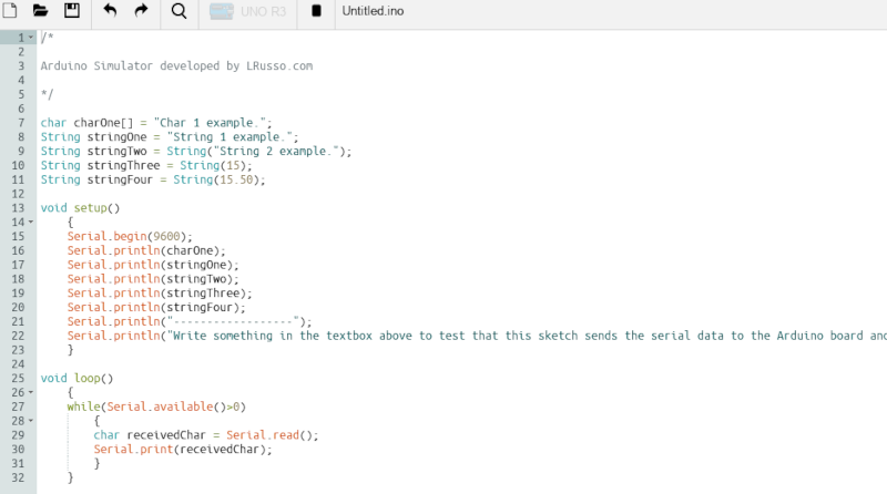
The software is available for Windows or Linux and the AVR/Arduino emulation is built in. For the PIC on Linux, you need an external software simulator that you can easily install. This is provided with the Windows version. You can see one of several videos available about an older release of the tool below. There is also a window that can compile your Arduino code and even debug it, although that almost always crashed for me after a few minutes of working. As you can see in the image above, though, it is capable of running some pretty serious Arduino code as long as you aren’t debugging.

Looks and sounds exciting, right? It is, but be sure to save often. Under Linux, it seems to crash pretty frequently even if you aren’t debugging. It also suffers from other minor issues like sometimes forgetting how to move components. Saving, closing the application, and reopening it seems to fix that. Plus, we assume they will squash bugs as they are reported. One of my major hangs was solved by removing the default (old) Arduino IDE and making sure the most recent was on the path. But the crashing was frequent and seemed more or less random. It seemed that I most often had crashes on Linux with occasional freezes but on Windows it would freeze but not totally crash.

Basic Operation

The basic operation is pretty much what you’d expect. The window is broadly divided into three panes. The leftmost pane shows, by default, a palette of components. You can use the vertical tab strip on the left to also pick a memory viewer, a property inspector, or a file explorer.

The central pane is where you can draw your circuit and it looks like a yellow piece of engineering paper with a grid. Along the top are file buttons that do things like save and load files.

You’ll see a similar row of buttons above the rightmost pane. This is a code editor and debugging window that can interface with the Arduino IDE. It looks like it can also interface with GCBasic for the PIC, although I didn’t try that.

You drag components from the left onto the circuit. Wiring isn’t a distinct operation. You just let the mouse float over the connection until the cursor makes a cross. Click and then drag to the connection point and click again. Sometimes the program forgets to make the cross cursor and then I’ve had to save and restart.

Most of the components are just what you think they are. There are some fun ones including a keypad, an LED matrix, text and graphic LCDs, and even stepper and servo motors. You’ll also find several logic functions, 7400-series ICs, and there are annotation tools like text and boxes at the very bottom. You can right click on a category and hide components you never want to see.

At the top, you can add a voltmeter, an ammeter, or an oscilloscope to your circuit. The oscilloscope isn’t that useful because it is small. What you really want to do is use a probe. This just shows the voltage at some point but you can right click on it and add the probe to the plotter which appears at the bottom of the screen. This is a much more useful scope option.

There are a few quirks with the components. The voltage source has a push button that defaults to off. You have to remember to turn it on or things won’t work well. The potentiometers were particularly frustrating. The videos of older versions show a nice little potentiometer knob and that appears on my Windows laptop, too. On Linux the potentiometer (and the oscilloscope controls) look like a little tiny joystick and it is very difficult to set a value. It is easier to right click and select properties and adjust the value there. Just note that the value won’t change until you leave the field.

Microcontroller Features

If that’s all there was to it, you’d be better off using any of a number of simulators that we’ve talked about before. But the big draw here is being able to plop a microcontroller down in your circuit. The system provides PIC and AVR CPUs that are supported by the simulator code it uses. There’s also four variants of Arduinos: the Uno, Nano, Duemilanove, and the Leonardo.

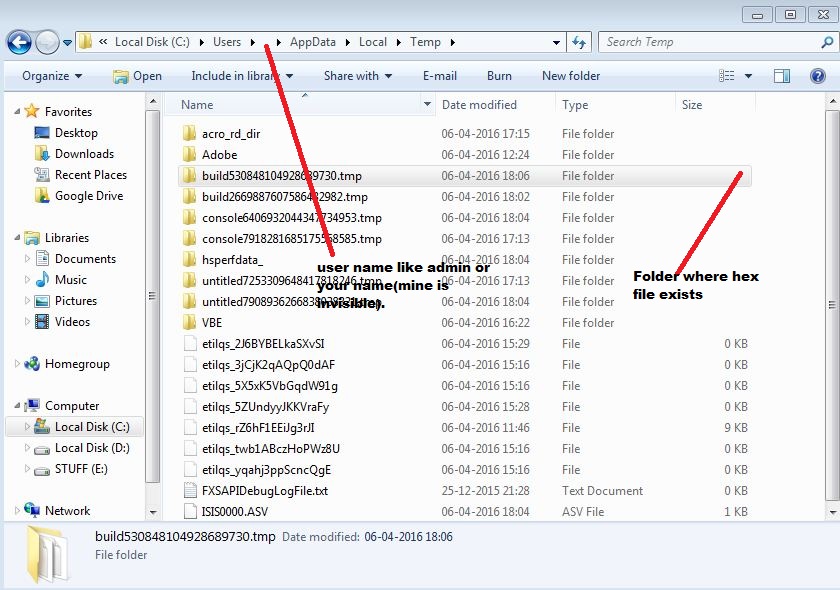
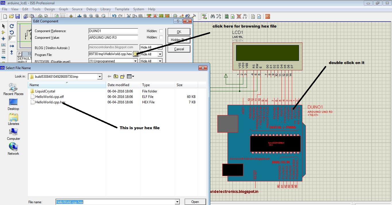
You can use the built-in Arduino IDE — just make sure you have the real Arduino software on your path and it is a recent version. Also, unlike the real IDE, it appears you must save your file before a download or debug will notice the changes. In other words, if you make a change and download, you’ll compile the code before the change if you didn’t save the file first. You don’t have to use the built-in IDE. You can simply right click on the processor and upload a hex file. Recent Arduino IDEs have an option to export a hex file, and that works with no problem.

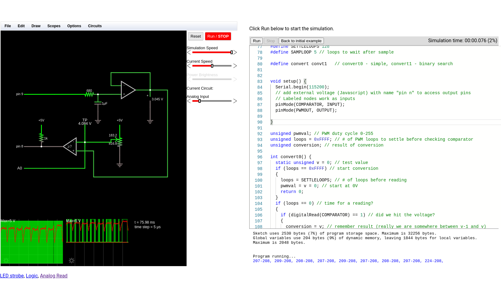
When you have a CPU in your design, you can right click it and open a serial monitor port which shows virtual serial output at the bottom of the screen and lets you provide input.

The debugging mode is simple but works until it crashes. Even without debugging, there is an option to the left of the screen to watch memory locations and registers inside the CPU.

Overall, the Arduino simulation seemed to work quite well. Connecting to the Uno pins was a little challenging at certain scales and I accidentally wired to the wrong pin on more than one occasion. One thing I found odd is that you don’t need to wire the voltage to the Arduino. It is powered on even if you don’t connect it.

Besides the crashing, the other issue I had was with the simulation speed which was rather slow. There’s a meter at the top of the screen that shows how slow the simulation is compared to real-time and mine was very low (10% or so) most of the time. There is a help topic explaining that this depends if you have certain circuit elements and ways to improve the run time, but it wasn’t bad enough that I bothered to explore it.

My first thought was that it would be difficult to handle a circuit with multiple CPUs in it since the debugging and serial monitors are all set up for a single CPU. However, as the video below shows, you can run multiple instances of the program and connect them via a serial port connection. The only issue would be if you had a circuit where both CPUs were interfacing with interrelated circuitry (for example, an op amp summing two signals, one from each CPU).

A Simple Example

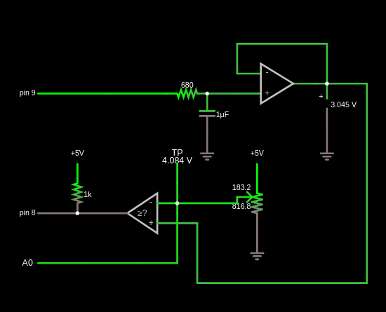
As an experiment, I created a simple circuit that uses an Uno. It generates two PWM signals, integrates them with an RC circuit and then either drives a load or drives a load through a bipolar emitter follower. A pot lets you set the PWM percentages which are compliments of each other (that is, when one is at 10% the other is at 90%). Here’s the circuit:

Along with the very simple code:

int v;

const int potpin=0;
const int led0=5;
const int led1=6;

void setup() {
Serial.begin(9600);
Serial.println("Here we go!");
}

void loop() {
int v=analogRead(potpin)/4;
Serial.println(v);
analogWrite(led0,v);
analogWrite(led1,255-v);
delay(250);
}

Note that if the PWM output driving the transistor drops below 0.7V or so, the transistor will shut off. I deliberately didn’t design around that because I wanted to see how the simulator would react. It correctly models this behavior.

There’s really no point to this other than I wanted something that would work out the analog circuit simulation as well as the Arduino. You can download all the files from GitHub, including the hex file if you want to skip the compile step.

If you use the built-in IDE on the right side of the screen, then things are very simple. You just download your code. If you build your own hex file, just right click on the Arduino and you’ll find an option to load a hex file. It appears to remember the hex file, so if you run a simulation again later, you don’t have to repeat that step unless you moved the hex file.

However, the IDE doesn’t remember settings for the plotter, the voltage switches, or the serial terminal. You’ll especially want to be sure the 5V power switch above the transistor is on or that part of the circuit won’t operate correctly. You can right click on the Arduino to open the serial monitor and right click on the probes to bring back the plotter pane.

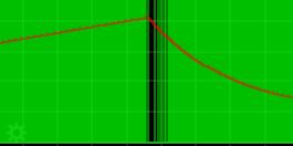
The red power switch at the top of the window will start your simulation. The screenshots above show close-ups of the plot pane and serial monitor.

Lessons Learned

This could be a really great tool if it would not crash so much. In all fairness, that could have something to do with my PC, but I don’t think that fully accounts for all of them. However, the software is still in pretty early development, so perhaps it will get better. There are a lot of fit and finish problems, too. For example, on my large monitor, many of the fonts were too large for their containers, which isn’t all that unusual.

The user interface seemed a little clunky, especially when you had to manipulate potentiometers and switches. Also, remember you can’t right-click on the controls but must click on the underlying component. In other words, the pot looks like a knob on top of a resistor. Right clicks need to go on the resistor part, not the knob. I also was a little put off that you can’t enter multiplier suffixes directly in component values. That is, you can’t enter a resistor value as 1K. You can enter 1000 or you can enter 1 and then change the units in a separate field to Kohms. But that’s not a big deal. You can get used to all of that if it would quit crashing.

I really wanted the debugging feature to work. While you can debug directly with simuavr or other tools, you can’t easily simulate all your I/O devices like you can with this tool. I’m hoping that becomes more robust in the future. Under Linux it would work for a bit and crash. On Windows, I never got it to work.

As I always say, though, simulation is great, but the real world often leads to surprises that don’t show up in simulation. Still, a simulation can help you clear up a host of problems before you commit to heating up the soldering iron or pulling out the breadboard. Simuide has the potential to be a great tool for simulating the kind of designs we see most on Hackaday.

If you want to explore other simulation options, we’ve talked a lot about LTSpice, including our Circuit VR series. There’s also the excellent browser-based Falstad simulator.

When it comes to building a neural network to simulate complex behavior, Arduino isn’t exactly the first platform that springs to mind. But when your goal is to model the behavior of an organism with only a handful of neurons, the constraints presented by an Arduino start to make sense.

It may be the most important non-segmented worm you’ve never heard of, but Caenorhabditis elegans, mercifully abbreviated C. elegans, is an important model organism for neurobiology, having had its entire nervous system mapped in 2012. [Nathan Griffith] used this “connectome” to simulate a subset of the diminutive nematode’s behaviors, specifically movements toward attractants and away from obstacles. Riding atop a small robot chassis, the Arduino sends signals to the motors when the model determines it’s time to fire the virtual worm’s muscles. An ultrasonic sensor stands in for the “nose touch” neurons of the real worm, and when the model is not busy avoiding a touch, it’s actively seeking something to eat using the “chemotaxis” behavior. The model is up on GitHub and [Nathan] hopes it provides an approachable platform for would-be neuroroboticists.

This isn’t the first time someone has modeled the nematode’s connectome in silico, but kudos to [Nathan] for accomplishing it within the constraints an Arduino presents.

The Santa Cruz Robotics Club met again today, for the first time in over a month.  The current project is not the underwater ROV (we’re all getting very tired of waterproofing problems), but an automated Nerf gun.

The club members came up with some very ambitious plans for the Nerf gun (which included getting a Raspberry Pi and doing image processing to have a self-aiming gun), but I’m making them build quick-and-easy prototypes to try out their ideas one step at a time.  I don’t think I can get an Raspberry Pi this summer—the companies doing the distribution aren’t taking more orders (just expressions of interest) and they don’t expect to clear the current backlog until September at the soonest.  They are doing batches of 100,000 units, and that doesn’t seem to be enough to shrink the lead time—if anything, the lead time is growing.

So, giving up on image processing for this summer, there are still a lot of things to build.  For today’s four-hour meeting (which included a 1-hour trip to the hardware store and a fifteen-minute snack break), the goal was simply to test out the basic launcher concept: an air reservoir pressurized by a bike pump, a solenoid valve, and a barrel.

The first prototype. The air reservoir is about 18″ of 1-½” PVC pipe on the left, and the barrel is about 24″ of ½” PVC pipe on the right.

The biggest problem was that the valve has ¾” male pipe threads, but we wanted 1-½” PVC pipe for the reservoir (because we had a piece handy—we may build a bigger reservoir later) and ½” PVC pipe for the barrel (because Nerf darts just fit inside—probably Nerf guns were prototyped with PVC barrels).  Our hardware store run was to get threaded adapters to make things fit.We wanted everything to be joined with screw threads, so that we could disassemble the components and replace them or add elbows as needed.

Note that the ½” PVC pipe is also a good size for compressed-air paper “rockets”.  The term “rocket” is a misnomer here, as all the acceleration occurs while the rocket is on the launcher—it is modeled more like a gun than like a rocket. (But my soda-bottle rocket simulator can model these paper bullets also.)  It would probably best to have a shorter barrel for doing rocket launching—just the length of the rocket and no more, since the longer barrel results in more pressure loss with no gain in launch speed.

The bicycle valve glued into a ½” female-threaded end cap was one I’ve had for a long time, as part of a soda-bottle rocket launcher. I had two of them, and both failed in testing today (the Barge cement holding the valve stem in failed—we’ve now reglued them with a different cement), though we managed some testing before the failure.

The solenoid valve we used was the same model (sold by Sparkfun) as the one used for the vacuum bottle on the ROV.  It has ¾” male pipe threads on each side.  To make it air-tight we had to disassemble it and grease the rubber membrane thoroughly with vaseline or faucet grease, but we had done that months ago, so it did not need to be done today.  The valve only works in one direction, but the high-pressure side is clearly marked by a metal intake screen, so assembling it the right way around is easy.

I was not sure that the solenoid valve would work in this application. It is not the model of valve that the compressed-air “rocket” people have used—those valves cost about twice as much and have female threaded ends rather than male threaded ends. I think that the mechanism they use may open up a bigger channel for air or water than the cheap solenoid valve sold by Sparkfun.

My first concern was that I did not know whether the valve would open up wide enough and fast enough to let a blast of air through to get a clean launch.  Second, I did not know whether we could open and close the valve fast enough to retain pressure in the reservoir for doing multiple shots.

We controlled the solenoid valve with an Arduino and the Hexmotor motor-control board (which is really overkill for one solenoid—a single power transistor would be enough to interface the Arduino to a solenoid, but I did not have one handy).  My son wrote an Arduino program to allow us to experiment with the duration of the solenoid pulse.  If it were too short, the Nerf dart would not leave the barrel.  If it were too long, air pressure would be wasted.  He allowed for 100 µsec increments in pulse duration, under control from commands on the USB serial line.

Because the glue they used takes 24 hours to set properly, we only tested at low pressure today (20–30 psi).  At those pressures, a 16 msec pulse was not long enough for the dart to clear the barrel, but a 19.2 msec pulse was easily long enough. We were also able to launch a 14g paper “rocket” left over from Maker Faire, though it did not go as high as the approximately 1.6g “Nerf” darts (I think several of the foam darts we have a different brand). We would not have expected it to go as high, since it was only accelerated for its 11″ length, not the 24″ length of the barrel for the darts, and it weighed a lot more.

One thing I thought about was monitoring the air pressure in the reservoir electronically. I doubt that we’ll put a pressure sensor in the reservoir, though, as the sensors I have only go up to 250 kPa absolute (about 21 psi above atmospheric pressure—about as low as we could fire with).  Freescale makes a 145psi (1000 kPa) sensor, the MPX5999D, but it is a differential sensor without port tubes (so would be difficult to mount) and it costs $13.

Perhaps the other thing worth doing today is to analyze how fast the Nerf dart should be going as it leaves the barrel, and how high it should fly if we shoot it straight up.  The physics here is fairly simple, if we assume that opening the solenoid valves connects us to a constant-pressure source. (In practice, we saw about a 10psi or 70kPa drop in pressure after one shot. If the pressure is P, then the force on the dart is P*area.  The cross-sectional area of the foam dart is a little hard to measure, because of the squishiness of the foam, but the inside diameter of the barrel is 1.45cm, for a cross-sectional area of 1.65 cm^2. At 140 kPa (about 20 psi), the force on the dart would be 23 Newtons.  That force is applied for about 60 cm (the length of the barrel), for a total energy of about 14 Joules.

We can use the kinetic energy of the dart to get its speed (E = ½ m v²), so for 140 kPa, the dart should leave the barrel at about 130 m/s or 290 mph. I suspect that we are not getting anywhere near that speed, for several reasons, including leakage of air around the dart, limited speed of air moving through the valve, and friction of the dart in the barrel (mainly from the pressure wave in front of it, but also from rubbing on the sides of the barrel).

We can also use the kinetic energy of the dart to estimate how high it would fly (ignoring air resistance, which is obviously hugely important for a low density object like a foam dart). The potential energy of a mass at height h is , so the height it would go without air resistance is . For 14 Joules and 1.6 grams, that would be almost 900m. I think that 20m is a more reasonable estimate for the height the dart went, though I never could see it near the top of its trajectory.

I tried adding the specs for the Nerf dart and a 60cm barrel to my rocket simulator (to get a crude estimate of the effect of air drag), and for 140 kPa I got an estimated max speed of 132m/s and an estimated max height of 52.6m. I don’t know if that height is reasonable—certainly it is better than the no-air-resistance estimate. The 6.78 second estimated time of flight seems to be fairly reasonable, though we never timed it.

Doubling the pressure increases the maximum velocity by a factor of 1.414, but only increases the maximum height to 60.8 m, a 16% increase. Doubling the barrel length has about the same effect. Air drag is what determines the speed of the dart, and that is the least well-modeled part of my simulation.

On Thursday, when they club meets again, they’ll try experimenting with higher pressures, and see whether 17 or 18 msec pulses are long enough—the shorter the pulse the less air will be wasted, and the more shots they can make from the reservoir.  It may be necessary to design a bigger reservoir or add a compressor to the design, since they eventually want a fully automatic Nerf gun, not the one-shot muzzle-loader that they made as the prototype today.  They’ll also start designing a pan-tilt mechanism for the Nerf gun, probably prototyping it out of Lego Technic components.