Physics Lab 2
The Physics Lab 1 post described a first experiment using ultrasonic rangefinders. The students have not really done the Wikipedia-style writeup of how an ultrasonic rangefinder works that I wanted. I’m not sure whether to push for that or to let it slide—it is important to develop technical reading and writing skills, but they have not yet gotten to the point in the physics course where they could actually derive the speed of sound equation. The speed of sound in a gas is only vaguely referred to in Chapter 12 of Matter and Interactions, though there is quite a bit on the speed of sound in a solid.
I ended up buying two different ultrasonic rangefinders:
- PING))) ultrasonic range finder(Note: parallax.com also has mounting brackets, servo-mount option for panning, and packages that combine the range finder with other sensors.)

Parallax PING))) sensor
- MaxBotix LV-MaxSonar-EZ2 MB1020
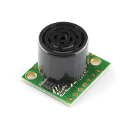
- MaxBotix rangefinder
Both of these rangefinders provide a pulse-width output that can be measured with the Arduino pulseIn function call. The measurement is provided in microseconds, but seems to have a slightly coarser resolution, with measurements spaced about 5 microseconds apart. To convert round-trip time into round-trip distance, we have to multiply the time in seconds by the speed of sound in meters/second.
There is an online calculator for the speed of sound as a function of temperature, pressure, and humidity, which gives a citation for the calculation (from the Journal of the Acoustical Society of America), but does not give a clear statement of calculation actually used. The same calculator (at least citing the same source) is also available from UK’s National Physical Lab. I used a simpler approximation (without humidity or pressure corrections) from Wikipedia’s Speed of Sound article:

On Friday, we did the lab itself:
- Hook up the rangefinder to the Arduino and program the Arduino to keep taking measurements and reporting them to the serial line. (I wrote the Arduino program myself, but my son is working on a Python program to record a series of measurements from the Arduino, which will be needed for the next lab.)
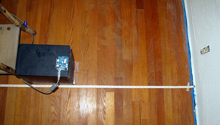
The setup for Lab 1. The Ping sensor is plugged directly into the Arduino, which sits on top of a copy of the OED, to get it far enough from the floor that we don't detect the floor rather than the wall.
- Calibrate the sensor by placing it at carefully measured distances from a hard wall and recording the readings. Repeat at several different distances. (Record temperature, humidity, and barometric pressure, if possible.) Here are the measurements made by the students, taking just the midpoint of the range observed:
# MaxBotix LV-MaxSonar-EZ Calibration
# Distance (centimeters) Delay Time (microseconds)
10 818
20 1075
30 1515
40 2299
50 2887
60 3470
70 4060
80 4645
90 5231
100 5815
# Parallax Ping))) Sensor Calibration
# Distance (centimeters) Delay Time (microseconds)
10 735
20 1215
30 1800
40 2405
50 3015
They had a lot of trouble getting consistent readings for the Ping))) sensor. I think that this may have been due to trying to take the measurements without pausing enough between them, so I added an extra millisecond delay after each Ping))) measurement, and my son and I collected new data today. We modified the setup slightly, so that instead of using a tape measure on the floor, we measured from the wall to the front of the Ping))) sensor with a steel tape measure. Here are the measurements we made:
# Ping))) calibration data
# 1 October 2011
# Arduino report several (usually 6) measurements for each distance
# We recorded the actual distance, the minimum and maximum reported time of flight,
# and the minimum and maximum distance reported by the Arduino.
# The reported distance assumed 343.21m/sec speed of sound, and that the time of flight
# was twice the distance.
#distance(cm) min_tof(usec) max_tof(usec) min_cm max_cm
10 616 624 10.57 10.71
20 1225 1230 21.02 21.11
30 1786 1818 30.65 31.20
40 2385 2391 40.93 41.03
50 2939 2962 50.44 50.83
60 3540 3542 60.75 60.78
70 4065 4089 69.76 70.17
80 4610 4729 79.11 81.15
90 5240 5265 89.92 90.35
100 5833 5858 100.10 100.53
110 6444 6446 110.58 110.62
120 7018 7050 120.43 120.98
130 7575 7582 129.99 130.11
These measurements were fairly consistent (though the variation is larger than I’d like). I did notice that the Ping))) sensor could get fooled rather badly when an object disappeared from its field of view. For example, when pointing the sensor at the ceiling from my benchtop, the distance is reported as a fairly consistent 177±0.5cm. Waving an object in front of the sensor got reasonable readings, but removing the object caused the sensor to get stuck reporting 50.5±1cm, though there was nothing at that distance. Sometimes the sensor returned to the 177cm reading, sometimes to the 50cm reading, and I’ve not been able to figure out what causes the difference. The MaxBotix sensor has different dropout problems, sometimes missing the echo and reporting a very long distance, but generally seems to be a little more stable.
What to do before next week’s lab
- Plot the sensor readings vs. the actual distance.
- Do linear regression to get a predictor of actual distance given sensor reading. (Caveat: need to plot distance vs. readings rather than readings vs. distance to get best fit for calibration.) What is the relationship between the speed of sound and the slope of the line?
- What is the accuracy and precision of the measurements? What range of distances can be measured? Is the accuracy better expressed in terms of absolute error (±5mm, for example) or relative error (±1%, for example)?
- Fix the Arduino program to get better estimates of the distances from the sensors, if possible.
- Get a recording program working to record a series of measurements of a moving object.
What to do in next week’s lab
- Redo the Maxbotix calibration the same way we redid the Ping))) calibration, collecting min and max time of flight and using better distance measurements.
- Use either the Ping))) or the Maxbotix sensor to record the movement of a simple object away from the sensor and plot the motion.
- Write a Vpython program that simulates the motion, using only a few constants, not a table of positions or velocities (that is, approximate the motion as constant velocity or constant acceleration). The simple object could be a small vehicle made from Lego (motorized or not), a mousetrap car, a rolling ball, a falling ball, or whatever else is easy to measure.
Other homework
- Read Chapter 2.
- Work problems 2P38, 2P40, 2P62, 2P63, 2P66, and 2P69.
- Do computational problem 2P72.
Tagged: Arduino, engineering education, Matter and Interactions, physics, rangefinder, science education, ultrasonic sensor